Download
1 / 38
380 likes | 388 Views
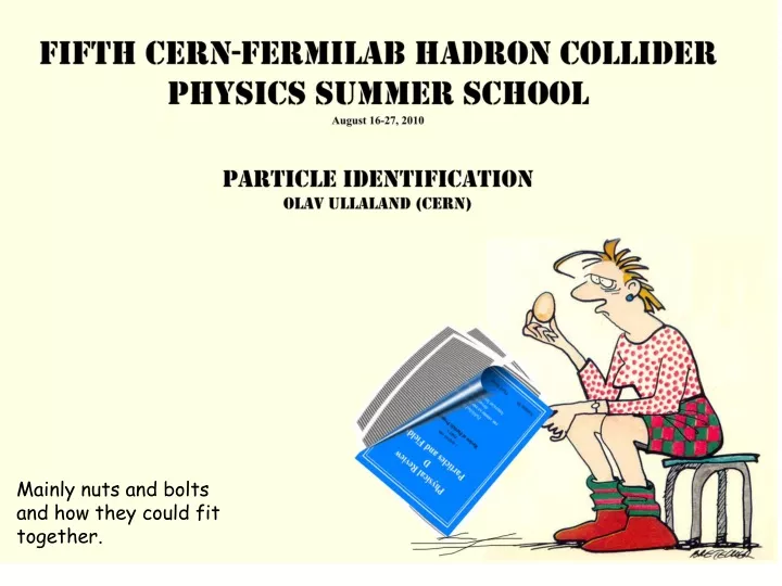
Mainly nuts and bolts and how they could fit together.

E N D
We will focus on charged particle identification as the detection and identification of neutral particles is covered in the Calorimeter lectures by Jane Nachtman. For particle Tracking see lecture of Michael Hildreth and Statistics and Systematics was given by Roger Barlow.
We will also have a look at where the real data is coming from and why.
We will not be concerned by all the charged particles which are around. We will just concentrate on those which have a lifetime long enough for us to observe them. That is: e, m, p, K, p. Main topics: - Time-of-Flight - Cherenkov - Transition radiation and a little - Muon - dE/dX The Pigeon Hole Principle. If you have fewer pigeon holes than pigeons and you put every pigeon in a pigeon hole, then there must result at least one pigeon hole with more than one pigeon. It is surprising how useful this can be as a proof strategy. First stated in 1834 by Peter Dirichlet (1805-1859) He got instant fame, not for this, but since his first publication concerned the famous Fermat's Last Theorem. The theorem claimed that for n > 2 there are no non-zero integers x, y, z such that xn + yn = zn. J J O'Connor and E F Robertson
Particle Identification Detectors are normally not stand-alone detectors. As a rule, they require that the momentum of the particle is measured by other means. And - of course - by measuring the momentum, the track is defined. "Other means" is usually called a magnet and if:
Why bother? No Particle Identification With Particle Identification (a) (b) The invariant mass spectrum in units of GeV/c for selected B± D0K± candidates, (a) before and (b) after information from the RICH detectors is introduced. Genuine B± D0K± candidates are shown in red while misidentified B± D0p± candidates are shown in yellow. Combinatoric events are shown in green. A. Powell, CERN-THESIS-2010-010 - Oxford : University of Oxford, 2009.
PID, or the physics signal could be drowned in combinatory background. With Particle Identification No Particle Identification But the right tool might be required.
The tools. Cherenkov radiation: Prompt signal, measure photon emission angle, calculate b. Detector: photon detector 150 to 1000 nm. Transition radiation: Prompt signal, measure photon energy, calculate g. Detector: (normally) X-ray >1 keV Time-of-Flight: measure time and flight path, calculate b. Detector: Any detector that can detect charged particles. dE/dX: measure (small) energy deposit Detector: Any detector that can detect charged particles. Muon: measure whatever survives in the muon filter. Detector: Any detector that can detect charged particles.
Scramjet Missile Sets Record for Mach 5 Flight Time Particle Identification by Time of Flight measurement. Awesome! maybe
Fig. 1. (a) Simplified side view of one of the spectrometer arms. (b) Time-of-flight spectrum of e+e- pairs and of those events with 3.0<m<3.2 GeV. (c) Pulse-height spectrum of e- (same for e+) of the e+e- pair. With Time-of-Flight to Nobel Prize. During the experiment, the time-of-flight of each of the hodoscopes and the Čerenkov counters, the pulse heights of the Čerenkov counters and of the lead-glass and shower counters, the single rates of all the counters together with the wire chamber signals, were recorded and continuously displayed on a storage/display scope. Nobel Lecture, 11 December, 1976
Time-of-Flight Measurements. Δp/p = 4· 10−3 l = 10m, Δl/l = 10−4 Δt = 50ps. The bars are ±1σ.
When considering how many s's are required, it can be helpful to remember that (almost) all secondary particles are p (and have a momentum around 2GeV/c) and then we have to dig out something interesting with a K or a p. Or - not confusing the p-issue with whatever the K or p is doing in the data set. Peter A. Carruthers (ed.), Hadronic multiparticle production
Δt = 50ps. Assuming a spectrometer with the following characteristics: Δp/p = 4· 10−3 l = 10m, Δl/l = 10−4 What time resolution is required to do a particle identification up to X GeV/c?
Winston Cone is a nonimaging off-axis parabola of revolution which will maximise the collection of incoming rays. Transient time spread is in the range of 1 ns. Read-out in both ends. After pulses. (This is not a Winston cone). Transfer efficiency in the range of 210-3 the rule of thumb dE/dxmin for a plastic scintillator is about 2 MeV cm2/g, or about 2 · 104 photons/cm. This number of photons will be greatly reduced due to: the attenuation length of the material, the losses out from the material. Time resolution of the order of 50 ps is reported (for reasonable large detectors).
Photoemission threshold Wph of various materials Ultra Violet (UV) Visible Infra Red(IR) GaAs TMAE,CsI Bialkali Multialkali TEA 12.3 4.9 3.1 2.24 1.76 1.45 E [eV] 100 250 400 550 700 850 l [nm] Photon detectors Main types of photon detectors: • gas-based • vacuum-based • solid-state • hybrid from T. Gys, Academic Training, 2005
S-20 (Sb-Na2-K-Cs) tri-alkaline photo cathode with quartz window. Ionisation potential Alkali bi-alkali Cs 3.894 eV Sb 8.64 K 4.341 Na 5.139 Photo-electric work function Cs 2.1 eV K 2.3 Na 2.8 Sb 4.8 Other alkalis have essentially the same scheme.
How to know when the signal was there. Time slewing and other evil things. Thanks to Hamamatsu and Burle.
ConstantFraction Discriminator. Comparison of threshold triggering (left) and constant fraction triggering (right) http://en.wikipedia.org/wiki/Constant_fraction_discriminator Operation of the cfd. The input pulse (dashed curve) is delayed (dotted) and added to an attenuated inverted pulse (dash-dot) yielding a bipolar pulse (solid curve). The output of the cfd fires when the bipolar pulse changes polarity which is indicated by time tcfd. Basic functional diagram of a constant fraction discriminator. The moment at which the threshold discriminator fires depends on the amplitude of the pulse. If the cable delay of the cfd is too short, the cfd fires too early (tcfd). For small input pulses, the timing is determined by the threshold discriminator and not by the cfd part. Martin Gerardus van Beuzekom, Identifying fast hadrons with silicon detectors (2006) Dissertaties - Rijksuniversiteit Groningen See also: Wolfgang Becker, Advanced time-correlated single photon counting techniques, Springer Berlin Heidelberg (January 14, 2010)
(A) (C) Pulse Height (ADC ch.) Slew-correction time, t cor, is defined as: where the constant A0 is normally evaluated for each PMT and ADC is the signal pulse height. s:55 ps Raw TOF (ns) Pulse Height (ADC ch.) ~4 MeV (D) (B) Time Resolution (ns) Pulse Height (ADC ch.) Pulse Height (ADC ch.) Slew corrected (ns) ~4 MeV Corrections for time slewing can also be done by measuring the apparent charge of the signal. (A) Pulse height distribution of one PM. (B) Rms time resolution as a function of pulse height . ADC channel 350 corresponds to an energy deposit of about 4 MeV. (C) Scatter plot of TOF(T-S1) and pulse height before slew correction. (D) Scatter plot of TOF(T-S1) and pulse height after slew correction. In a similar approach, Time-over-Threshold (ToT), can be used for time slewing correction. T. Kobayashi and T. Sugitate, Test of Prototypes for a Highly Segmented TOF Hodoscope, Nucl. Instrum. Methods Phys. Res., A: 287 (1990) 389-396
The clock issue. It is challenging to issue a high frequency clock to a large distributed system without falling into traps of slewing, power requirements, length of strips across the cell .... We will use the proposed NA62 experiment at CERN as an example. For more information see: http://na62.web.cern.ch/NA62/ http://na62.web.cern.ch/NA62/Documents/Chapter_3-3_GTK_V1.4.3.pdf
The aim of NA62: to extract a 10% measurement of the CKM parameter |Vtd|. hit correlation via matching of arrival times – 100 ps GTK seesall particles selects particleswith 75 GeV/c RICH identifies pions straw chambers measure position seeskaons only Mag2 Mag3 straw chambers RICH GTK3 GTK1 Cedar GTK2 Achromat Mag1 Mag4 250 m Vacuum tank A. Kluge, PE/ESE, CERN beam: hadrons, only 6% kaons0.06 only 20% of charged kaon decay in the vacuum tank 0.20 out of which only 10-11 decays are of interest10-11decay into one pion, one neutrino and one anti-neutrino total probability1.2 10-13
amplifier discriminator/ time-walk-compensator buffering TDC amplifier & discriminator/ time-walk-compensator time-to-digital converter TDC buffering & read-out processor buffering & read-out processor reference clock A. Kluge, PE/ESE, CERN
t1 t2 U1 k2 k1 n 0 n-1 1 t0 .. tclk tclk Wilkinson Time toDigitalConverter(dual slope) and then: Related solutions with Delay Locked Loop and Phase Locked Loop A. Kluge, PE/ESE, CERN
MRPC:1013Wcm Two very different approaches to an especially good time resolution. J. Va’vra et al., Nucl. Instrum. Methods Phys. Res., A: 572 (2007) 459-462 A.N. Akindinov et al., Nucl. Instrum. Methods Phys. Res., A: 533 (2004) 74-78
One thing is to have a signal, another thing is to know where the signal is. Some things to look (out) for. Will follow B. Zagreev at ACAT2002, 24 June 2002 http://acat02.sinp.msu.ru/ • High multiplicity dN/dY8000 primaries • (12000 particles in TOF angular acceptance) • 45(35)% of them reach TOF, but they produce a lot of secondaries • High background • total number of fired pads ~ 25000 occupancy=25000/160000=16% • but only 25% of them are fired by particles having track measured by TPC • Big gap between tracking detector (TPC) and TOF • big track deviation due to multiple scattering ALICE Time-of-Flight detector R=3.7 m S=100 m2 N=160000 • Tracking (Kalman filtering) • Matching • Time measurements • Particle identification
Combinatorial algorithm for t0 calculation. 1. Consider a very small subset (n) of primary Let l1…ln, p1…pn, t1…tn- be length, momentum and time of flight of corresponding tracks. Now we can calculate the velocity (vi) of particle i by assuming that the particle is p, K or p. 2. Then we can calculate time zero: 3. We chose configuration C with minimal
Which gives, with simulated events, particle identification with simple 1D or 2D cuts: Neural network and Probability approach will of course also be used.
y gK(x,y)~gK(x)gK(y) 1D cuts gK(y) kaons pions 2D cut gK(x) x If you have Detector X and your friend has Detector y recording data of the same event:
σTOF=σ/√2 = 88 ps β With real data:
Assume a sample of n uncorrelated measurements xi. Let the series be ordered such that x1<x2< ... Then the cumulative distribution is defined as: 0 x < x1 Sn(x)= i/n xi x < xi+1 1 x xn The theoretical model gives the corresponding distribution F0(x) The null hypothesis is then H0: Sn(x)=F0(x) The statistical test is: Dn=max|Sn(x)-F0(x)| Example In 30 events measured proper flight time of the neutral kaon in K0 p+e-n which gives: D30=max|S30(t)-F0(t)|=0.17 or ~50% probability The same observations by c2method. n observations of x belonging to N mutually exclusive classes. H0 : p1=p01, p2=p02, ... , pN=p0N for Sp0i=1 Test statistic: when H0 is true, this statistic is approximately c2 distributed with N-1 degrees of freedom. c2(obs)=3.0 with 3 degrees of freedom or probability of about 0.40 - Kolmogorov-Smirnov testsFrodesen et al., probability and statistics in particle physics, 1979 There is more to it than what is written here!
y=a x + b a=-2 b=20 =1 y=a x + b a=1 b=-17 =1 x cosQ+y sinQ = r This point-to-curve transformation is the Hough transformation for straight lines The Hough transform is a technique which can be used to isolate features of a particular shape within an image. The Hough technique is particularly useful for computing a global description of a feature(s) (where the number of solution classes need not be known a priori), given (possibly noisy) local measurements. The motivating idea behind the Hough technique for line detection is that each input measurement (e.g. coordinate point) indicates its contribution to a globally consistent solution (e.g. the physical line which gave rise to that image point). from http://homepages.inf.ed.ac.uk/rbf/HIPR2/hough.htm
Ring Finding with a Markov Chain. Sample parameter space of ring position and size by use of a Metropolis Metropolis-Hastings Markov Chain Monte Carlo (MCMC) Interested people should consult: C.G. Lester, Trackless ring identification and pattern recognition in Ring Imaging Cherenkov (RICH) detectors, NIM A 560(2006)621-632 http://lhcb-doc.web.cern.ch/lhcb-doc/presentations/conferencetalks/postscript/2007presentations/G.Wilkinson.pdf G. Wilkinson, In search of the rings: Approaches to Cherenkov ring finding and reconstruction in high energy physics, NIM A 595(2008)228 W. R. Gilks et al., Markov chain Monte Carlo in practice, CRC Press, 1996 Example of 100 new rings proposed by the “three hit selection method” for consideration by the MHMC for possible inclusion in the final fit. The hits used to seed the proposal rings are visible as small black circles both superimposed on the proposals (left) and on their own (right). It is not about Markov chain, but have a look in M.Morháč et al., Application of deconvolution based pattern recognition algorithm for identification of rings in spectra from RICH detectors, Nucl.Instr. and Meth.A(2010),doi:10.1016/j.nima.2010.05.044
Kalman filter The Kalman filter is a set of mathematical equations that provides an efficient computational (recursive) means to estimate the state of a process, in a way that minimizes the mean of the squared error. The filter is very powerful in several aspects: it supports estimations of past, present, and even future states, and it can do so even when the precise nature of the modelled system is unknown. http://www.cs.unc.edu/~welch/media/pdf/kalman_intro.pdf iweb.tntech.edu/fhossain/CEE6430/Kalman-filters.ppt R. Frühwirth, M. Regler (ed), Data analysis techniques for high-energy physics, Cambridge University Press, 2000 07/10/2009 US President Barack Obama presents the National Medal of Science to Rudolf Kalman of the Swiss Federal Institute of Technology in Zurich during a presentation ceremony for the 2008 National Medal of Science and the National Medal of Technology and Innovation October 7, 2009 in the East Room of the White House in Washington, DC. 2008 Academy Fellow Rudolf Kalman, Professor Emeritus of the Swiss Federal Institute of Technology in Zurich, has been awarded the Charles Stark Draper Prize by the National Academy of Engineering. The $500,000 annual award is among the engineering profession’s highest honors and recognizes engineers whose accomplishments have significantly benefited society. Kalman is honored for “the development and dissemination of the optimal digital technique (known as the Kalman Filter) that is pervasively used to control a vast array of consumer, health, commercial, and defense products.”
Pion-Kaon separation for different PID methods. The length of the detectors needed for 3s separation. The same as above, but for electron-pion separation. Dolgoshein, NIM A 433 (1999)