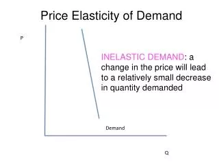
Download
1 / 37
370 likes | 377 Views
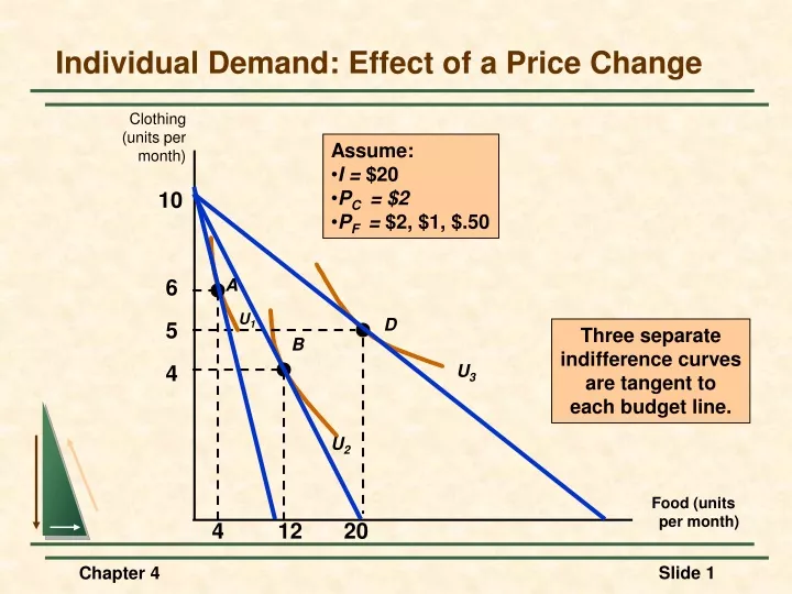
Assume: I = $20 P C = $2 P F = $2, $1, $.50. 10. 6. A. U 1. D. 5. Three separate indifference curves are tangent to each budget line. B. 4. U 3. U 2. 4. 12. 20. Individual Demand: Effect of a Price Change. Clothing (units per month). Food (units per month).

E N D
Assume: • I = $20 • PC = $2 • PF = $2, $1, $.50 10 6 A U1 D 5 Three separate indifference curves are tangent to each budget line. B 4 U3 U2 4 12 20 Individual Demand: Effect of a Price Change Clothing (units per month) Food (units per month) Chapter 4
Individual Demand: Effect of a Price Change The price-consumption curve traces out the utility maximizing market basket for the various prices for food. Clothing (units per month) 6 A Price-Consumption Curve U1 D 5 B 4 U3 U2 Food (units per month) 4 12 20 Chapter 4
Individual Demand: Effect of a Price Change The Individual Demand Curve: 2 Important Properties 1) The level of utility that can be attained changes as we move along the curve. 2) At every point on the demand curve, the consumer is maximizing utility by satisfying the condition that the MRS of food for clothing equals the ratio of the prices of food and clothing. Chapter 4
When the price falls: Pf/Pc & MRS also fall E $2.00 • E: Pf/Pc = 2/2 = 1 = MRS • G: Pf/Pc = 1/2 = .5 = MRS • H:Pf/Pc = .5/2 = .25 = MRS G $1.00 Demand Curve $.50 H 4 12 20 Individual Demand: Effect of a Price Change Price of Food Food (units per month) Chapter 4
Income-Consumption Curve 7 D U3 5 U2 B 3 U1 A 4 10 16 Individual Demand: Effect of Income Changes Clothing (units per month) Assume: Pf = $1 Pc = $2 I = $10, $20, $30 An increase in income, with the prices fixed, causes consumers to alter their choice of market basket. Food (units per month) Chapter 4
E G H $1.00 D3 D2 D1 4 10 16 Individual Demand: Effect of Income Changes Price of food An increase in income, from $10 to $20 to $30, with the prices fixed, shifts the consumer’s demand curve to the right. Food (units per month) Chapter 4
Individual Demand: Effect of Income Changes Normal Good vs. Inferior Good • Income Changes • When the income-consumption curve has a positive slope, the quantity demanded increases with income; the income elasticity of demand is positive. The good is a normal good. • When the income-consumption curve has a negative slope, the quantity demanded decreases with income; the income elasticity of demand is negative. The good is an inferior good. Chapter 4
15 Income-Consumption Curve Both hamburger and steak behave as a normal good, between A and B... C 10 U3 …but hamburger becomes an inferior good when the income consumption curve bends backward between B and C. B 5 U2 A U1 5 10 20 30 Individual Demand: Effect of Income Changes with an Inferior Good Steak (units per month) Hamburger (units per month) Chapter 4
Individual Demand: Effect of Income Changes • Engel Curves • Engel curves relate the quantity of good consumed to income. • If the good is a normal good, the Engel curve is upward sloping. • If the good is an inferior good, the Engel curve is downward sloping. Chapter 4
Engel curve slopes upward for a normal good. Engel Curves: Normal Good Income ($ per month) 30 20 10 Food (units per month) 0 4 8 12 16 Chapter 4
Inferior Engel curve is backward bending for inferior goods. Normal Engel Curves: Inferior Good Income ($ per month) 30 20 10 Food (units per month) 0 4 8 12 16 Chapter 4
Individual Demand: Substitutes and Complements • Substitute goods: an increase (decrease) in the price of one leads to an increase (decrease) in the quantity demanded of the other. E.g. movie tickets and video rentals • Complements: an increase (decrease) in the price of one leads to a decrease (increase) in the quantity demanded of the other. E.g. gasoline and motor oil • Two goods are independent when a change in the price of one good has no effect on the quantity demanded of the other. Chapter 4
Income and Substitution Effects • A fall in the price of a good has two effects: • Substitution Effect: consumers will tend to buy more of the good that has become relatively cheaper, and less of the good that is now relatively more expensive. • Income Effect: consumers experience an increase in real purchasing power when the price of one good falls. Chapter 4
Income and Substitution Effects • Substitution Effect • The substitution effect is the change in an item’s consumption associated with a change in the price of the item, with the level of utility held constant. • When the price of an item declines, the substitution effect always leads to an increase in the quantity of the item demanded. Chapter 4
Income and Substitution Effects • Income Effect • The income effect is the change in an item’s consumption due to an increase in purchasing power, with the price of the item held constant. • If income increases, the quantity demanded for the product may increase or decrease. Even with inferior goods, the income effect is rarely large enough to outweigh the substitution effect. Chapter 4
When the price of food falls, consumption increases by F1F2 as the consumer moves from A to B. R The substitution effect,F1E, (from point A to D), changes the relative prices but keeps utility (satisfaction) constant. C1 A The income effect, EF2, ( from D to B) keeps relative prices constant but increases purchasing power. D B C2 U2 Substitution Effect U1 F1 E S F2 T Total Effect Income Effect Income and Substitution Effects: Normal Good Clothing (units per month) Food (units per month) O Chapter 4
As food is an inferior good in this example, the income effect is negative. However, the substitution effect is larger than the income effect. B U2 Total Effect Income Effect Income and Substitution Effects: Inferior Good Clothing (units per month) R A D Substitution Effect U1 Food (units per month) O F1 E S F2 T Chapter 4
From Individual to Market Demand: Determining the Market Demand Curve Price Individual A Individual B Individual C Market ($) (units) (units) (units) (units) 1 6 10 16 32 2 4 8 13 25 3 2 6 10 18 4 0 4 7 11 5 0 2 4 6 Chapter 4
The market demand curve is obtained by summing the consumer’s demand curves Market Demand DA DB DC Summing to Obtain a Market Demand Curve Price 5 4 3 2 1 Quantity 0 5 10 15 20 25 30 Chapter 4
Market Demand: Elasticity • Elasticity of Demand Recall: Price elasticity of demand measures the percentage change in the quantity demanded resulting from a 1% change in price. Chapter 4
Price Elasticity and Consumer Expenditure Demand If Price Increases, If Price Decreases, Expenditures: Expenditures: Inelastic (Ep<1)Increase Decrease Unit Elastic (Ep = 1) Are unchanged Are unchanged Elastic (Ep >1) Decrease Increase Chapter 4
Market Demand: Elasticity • Point Elasticity of Demand • Point elasticity measures elasticity at a point on the demand curve. • For large price changes (e.g. 20%), the value of the elasticity will depend upon where the price and quantity lie on the demand curve. • Problem: we may need to calculate price elasticity over a portion of the demand curve rather than at a single point. The price and quantity used as the base will alter the price elasticity of demand. Chapter 4
Market Demand: Elasticity Point Elasticity of Demand (An Example) • Assume • As price increases from $8 to $10, the quantity demanded falls from 6 to 4 • Percent change in price equals: $2/$8 = 25% or $2/$10 = 20% • Percent change in quantity equals: -2/6 = -33.33% or -2/4 = -50% • Elasticity equals: -33.33/25 = -1.33 or -50/20 = -2.5 • Which one is correct? Chapter 4
Market Demand: Elasticity • Arc Elasticity of Demand • Arc elasticity calculates elasticity over a range of prices • Its formula is: Chapter 4
Market Demand: Elasticity • Arc Elasticity of Demand (An Example) Chapter 4
An Example: Aggregate Demand For Wheat • The demand for US wheat is comprised of domestic demand and export demand. • The domestic demand for wheat is given by: • QDD = 1700 - 107P • The export demand for wheat is given by: • QDE = 1544 - 176P • Domestic demand is relatively price inelastic (-0.2), while export demand is more price elastic (-0.4). Chapter 4
Total world demand is the horizontal sum of the domestic demand AB and export demand CD. A C E Total Demand Export Demand Domestic Demand F D B The Aggregate Demand For Wheat Price ($/bushel) 20 18 16 14 12 10 8 6 4 2 Wheat(million bushels/yr.) 0 1000 2000 3000 4000 Chapter 4
Consumer Surplus • Consumer Surplus: the difference between the maximum amount a consumer is willing to pay for a good and the amount actually paid. • Combining consumer surplus with the aggregate profits that producers obtain we can evaluate: 1) Costs and benefits of different market structures 2) Public policies that alter the behavior of consumers and firms Chapter 4
The consumer surplus of purchasing 6 concert tickets is the sum of the surplus derived from each one individually. Market Price Consumer Surplus Price ($ per ticket) 20 19 18 17 16 Consumer Surplus 6 + 5 + 4 + 3 + 2 + 1 = 21 15 14 13 Rock Concert Tickets 0 1 2 3 4 5 6 Chapter 4
Consumer Surplus Market Price Demand Curve Actual Expenditure Consumer Surplus Price ($ per ticket) Consumer Surplus for the Market Demand 20 19 18 17 16 15 14 13 Rock Concert Tickets 0 1 2 3 4 5 6 Chapter 4
Network Externalities • Up to this point we have assumed that people’s demands for a good are independent of one another. • In fact, a person’s demand may be affected by the number of other people who have purchased the good. If this is the case, a network externality exists. Chapter 4
Positive Network Externalities • Positive network externality: the quantity of a good demanded by a consumer increases in response to an increase in purchases by other consumers. • The Bandwagon Effect • This is the desire to be in style, to have a good because almost everyone else has it, or to indulge in a fad. • This is the major objective of marketing and advertising campaigns (e.g. toys, clothing). Chapter 4
Positive Network Externality: Bandwagon Effect Price ($ per unit) D20 D40 D60 D80 D100 The market demand curve is found by joining the points on the individual demand curves. It is relatively more elastic. Demand Quantity (thousands per month) 20 40 60 80 100 Chapter 4
Positive Network Externality: Bandwagon Effect Suppose the price falls from $30 to $20. With no bandwagon effect, Qd would increase to 48,000 only. But as more people buy the good, it becomes stylish to own it and Qd increases further. Price ($ per unit) D20 D40 D60 D80 D100 $30 Demand $20 Pure Price Effect Bandwagon Effect Quantity (thousands per month) 20 40 60 80 100 48 Chapter 4
Negative Network Externalities • If the network externality is negative, a snob effect exists = the desire to own exclusive or unique goods. • The quantity demanded of a “snob” good is higher the fewer the people who own it. Chapter 4
Originally demand is D2, when consumers think 2000 people have bought a good. Demand $30,000 However, if consumers think 4,000 people have bought the good, demand shifts from D2 to D4 and its snob value has been reduced. $15,000 D2 D4 D6 D8 2 4 6 8 14 Pure Price Effect Negative Network Externality: Snob Effect Price ($ per unit) Quantity (thousands per month)
Negative Network Externality: Snob Effect Price ($ per unit) Demand is less elastic and as a snob good, its value is greatly reduced if more people own it. Sales decrease as a result. Examples: Rolex watches and long lines at the ski lift. Demand $30,000 Net Effect Snob Effect $15,000 D2 D4 D6 D8 Quantity (thousands per month) 2 4 6 8 14 Pure Price Effect