JPEG Compression

1. JPEG Compression CSC361/661 Spring 2002 Burg/Wong

2. Fact about JPEG Compression • JPEG stands for Joint Photographic Experts Group • JPEG compression is used with .jpg and can be embedded in .tiff and .eps files. • Used on 24-bit color files. • Works well on photographic images. • Although it is a lossy compression technique, it yields an excellent quality image with high compression rates.

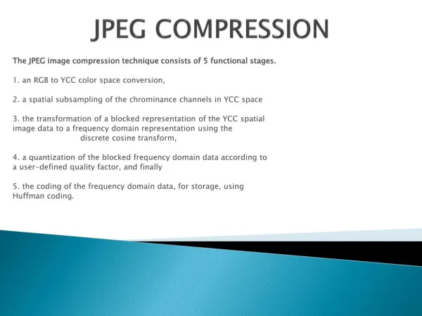
3. Steps in JPEG Compression • 1. (Optionally) If the color is represented in RGB mode, translate it to YUV. • 2. Divide the file into 8 X 8 blocks. • 3. Transform the pixel information from the spatial domain to the frequency domain with the Discrete Cosine Transform. • 4. Quantize the resulting values by dividing each coefficient by an integer value and rounding off to the nearest integer. • 5. Look at the resulting coefficients in a zigzag order. Do a run-length encoding of the coefficients ordered in this manner. Follow by Huffman coding.

4. Step 1a: Converting RGB to YUV • YUV color mode stores color in terms of its luminance (brightness) and chrominance (hue). • The human eye is less sensitive to chrominance than luminance. • YUV is not required for JPEG compression, but it gives a better compression rate.

5. Step 1a: Converting RGB to YUV • You can consider picture 3 pictures or three layers, one for each simple (YUV) as next

6. RGB vs. YUV • It’s simple arithmetic to convert RGB to YUV. The formula is based on the relative contributions that red, green, and blue make to the luminance and chrominance factors. • There are several different formulas in use depending on the target monitor. For example: Y = 0.299 * R +0.587 * G +0.114 * B U = -0.1687 * R – 0.3313* G + 0.5 * B +128 V = 0.5 * R – 0.4187 * G – 0.813 * B + 128

7. Example • Convert pixel value (734AF×0) from group of RGB to YUV group. Solution R = 0x07 =7 G = 0x34 =52 B = 0xAF = 175 By using YUV equation Y=50.8 V=124.2 U=-43.8

8. Step 1b: Downsampling • The chrominance information can (optionally) be downsampled. • The notation 4:1:1 means that for each block of four pixels, you have 4 samples of luminance information (Y), and 1 each of the two chrominance components (U and V). MCU – minimum coded unit Y Y U, V Y Y

9. Step 2: Divide into 8 X 8 blocks • وقد اختيرت مجموعة الألوان YUV وأحياناً YIQ (Y=luma, I=In-phase, Q=qudrature) لأن عنصرY يمثل الإضاءة، وذلك للاستفادة من ضعف حساسية العين للتغير في الألوان بعكس الإضاءة. فنستطيع اختصار الطبقة الثانية والثالثة Q و Iأو U و V لكل وحدة، لتكون بحجم 4×4 بيكسل بدل من 8×8 بيكسل، لتغطي كل بيكسل مساحة 2×2 بيكسل في الصورة الأصلية، كما في الشكل

10. Step 2: Divide into 8 X 8 blocks • Note that with YUV color, you have 16 pixels of information in each block for the Y component (though only 8 in each direction for the U and V components). • If the file doesn’t divide evenly into 8 X 8 blocks, extra pixels are added to the end and discarded after the compression. • The values are shifted “left” by subtracting 128. (See JPEG Compression for details.)

11. JPEG(Intraframe coding) • First generation JPEG uses DCT+Run length Huffman entropy coding. • Second generation JPEG (JPEG2000) uses wavelet transform + bit plane coding + Arithmetic entropy coding.

12. Discrete Cosine Transform • The DCT transforms the data from the spatial domain to the frequency domain. • The spatial domain shows the amplitude of the color as you move through space • The frequency domain shows how quickly the amplitude of the color is changing from one pixel to the next in an image file.

13. Step 3: DCT • The frequency domain is a better representation for the data because it makes it possible for you to separate out – and throw away – information that isn’t very important to human perception. • The human eye is not very sensitive to high frequency changes – especially in photographic images, so the high frequency data can, to some extent, be discarded.

14. DCT basis patterns

15. DCT example (only take 6 of 64 coefficients to reconstruct)

16. DCT coefficient

17. Step 3: Forward DCT For an N X N pixel image the DCT is an array of coefficients where where

18. Step 3: DCT • The color amplitude information can be thought of as a wave (in two dimensions). • You’re decomposing the wave into its component frequencies. • For the 8 X 8 matrix of color data, you’re getting an 8 X 8 matrix of coefficients for the frequency components.

19. Fourier Transform (p. 42 in your book)

20. Basic Functions for Discrete Cosine Transform

21. Step 4: Quantize the CoefficientsComputed by the DCT • The DCT is lossless in that the reverse DCT will give you back exactly your initial information (ignoring the rounding error that results from using floating point numbers.) • The values from the DCT are initially floating-point. • They are changed to integers by quantization. • See JPEG Compression for an example.

22. Step 4: Quantization • Quantization involves dividing each coefficient by an integer between 1 and 255 and rounding off. • The quantization table is chosen to reduce the precision of each coefficient to no more than necessary. • The quantization table is carried along with the compressed file.

23. Q (Quantization) • Divide all DCT coefficients by integer (quantization table) • Lossy compression • Only few and significant coefficients are left

24. Quantization example  After Q

25. Step 5: Arrange in “zigzag” order • This is done so that the coefficients are in order of increasing frequency. • The higher frequency coefficients are more likely to be 0 after quantization. • This improves the compression of run-length encoding. • Do run-length encoding and Huffman coding.

26. Step 5: Arrange in “zigzag” order

27. Zig-zag scan • Non-zero coefficients are grouped together.

28. Final step • In this stage we see the data of picture as a sequence of symbols especially zeros, which act content of picture with high frequencies which eye can detected in normal and then to get high compression we can used one of lossless compression ( RLE or Huffman)