Download
1 / 11
110 likes | 219 Views
MuTr LL1 simulation. Kazuya Aoki Kyoto Univ. MuTr LL1 overview. Using 3 stations (radial strips) one cathode plane from each station No Anode wire readout MuTrLL1 X MuIDLL1 in GL1 level No MuID road (symset) matching. Cosmic ray. MuTr LL1. MuTr. signal. MuTr test chamber at Kyoto.

E N D
MuTr LL1 simulation Kazuya Aoki Kyoto Univ.
MuTr LL1 overview • Using 3 stations (radial strips) • one cathode plane from each station • No Anode wire readout • MuTrLL1 X MuIDLL1 in GL1 level • No MuID road (symset) matching
Cosmic ray MuTr LL1 MuTr signal MuTr test chamber at Kyoto. Amp-shaper-discri Hit pattern Programmable Circuit (FPGA) MuTr LL1 140cm
choose hit strip charge 二値化 Discri. • Charge is induced 2 or 3 consecutive strips. • Discriminate the signals • Choose the center strip as the hit • The difference between peak strip and center strip is <=1 • This is gives enough resolution Thresh. Choose the center strip As the hit REAL DATA counts The difference
Algorithm m+ m- • Making lookup table for station1 & 3 • Calculate sagitta and make a decision! INPUT: single m 15GeV/c vertex z=0 sagitta: the difference between The actual hit at station#2 and interpolated position
1.Making lookup table m+ m- • For each strip at St#1 • get hit strip dist. at St#3 • Fit with gaus func. • get lower and upper limit • (+/- 3s from mean) • To reduce the data size • Collect all lower and upper limits and fit with straight line INPUT: single m 15GeV/c vertex z=0 For each strip at St#1 Upper limit lower limit Upper limit Fit with straight line Lower limit
Simulation procedure(event generator) Inclusive charged hadron pT spectra • Software and PDF • PYTHIA Ver6 • CTEQ5M1 • Settings for background • <kT>=2.5GeV/c , kT<10GeV/c • MSEL=2(MinBias : total s) • No cuts applied • 1M events • Agrees well with UA1 data • Settings for signal • MSEL=12 • Cuts applied • W should decay into m • The m should have PT>20GeV/c and -1.2>h>-2.2 or 1.2<h<2.4 • 50k events pp sqrt s = 200GeV pp sqrt s = 500GeV
Simulation procedurePISA Fitted func. (gaus) • Vertex distribution • rms of z = 17 • Run Number = 92446 • Dead area due to FEMs included • Dead area due to HV NOT INCLUDED BBC Z vertex RUN92446(REAL DATA) ( if you use Run Number -1 the induced charge is too large compared to the real data.)
MinBias(Total s) # of triggered events (MuTrLL1 X MuIDLL1) Definitions • Rejection Factor • Efficiency # of triggered events (MuTrLL1 x MuIDLl1) W decays into m which satisfy the following: pT>20GeV/c and -1.2>h>-2.2 or 1.2<h<2.4
Rejection & Efficiency Using only 2 stations Using 3 stations ( MuTr LL1 x MuID LL1) Eff = [MuIDLL1] x [MuTr acc] x [MuTr plane eff.] X [MuTr live area] = 66% 95% 79% 96%
Conclusion • Using 3 stations • We can get enough RF ( 23700 ) • Reading Anode wires might help to some extent when we only read 2 stations. • How can I get the indeced charge in wires?