Download
1 / 33
370 likes | 919 Views
Chapter 8 - Project Management Chapter Topics. The Elements of Project Management The Project Network Probabilistic Activity Times Project Crashing and Time-Cost Trade-Off Formulating the CPM/PERT Network as a Linear Programming Model. Project Management Overview.

E N D
Chapter 8 - Project ManagementChapter Topics • The Elements of Project Management • The Project Network • Probabilistic Activity Times • Project Crashing and Time-Cost Trade-Off • Formulating the CPM/PERT Network as a Linear Programming Model Chapter 8 - Project Management
Project ManagementOverview • Uses networks for project analysis. • Networks show how projects are organized and are used to determine time duration for completion. • Network techniques used are • - CPM (Critical Path Method) • - PERT (Project Evaluation and Review Technique) • Developed during late 1950s. Chapter 8 - Project Management
The Elements of Project Management • Management is generally perceived as concerned with planning, organizing, and control of an ongoing process or activity. • Project Management is concerned with control of an activity for a relatively short period of time after which management effort ends • Primary elements of Project Management to be discussed: • - Project team • - Project planning • - Project control. Chapter 8 - Project Management
The Elements of Project ManagementThe Project team • Project team typically consists of a group of individuals from various areas in an organization and often includes outside consultants. • Members of engineering staff often assigned to project work. • Most important member of project team is the project manager. • Project manager is often under great pressure because of uncertainty inherent in project activities and possibility of failure. • Project manager must be able to coordinate various skills of team members into a single focused effort. Chapter 8 - Project Management
Project Planning: PERT/CPM • PERT • Program Evaluation and Review Technique • Developed by U.S. Navy for Polaris missile project • Developed to handle uncertain activity times • CPM • Critical Path Method • Developed by Du Pont & Remington Rand • Developed for industrial projects for which activity times generally were known • Today’s project management software packages have combined the best features of both approaches. Chapter 8 - Project Management
PERT/CPM • PERT and CPM have been used to plan, schedule, and control a wide variety of projects: • R&D of new products and processes • Construction of buildings and highways • Maintenance of large and complex equipment • Design and installation of new systems Chapter 8 - Project Management
PERT/CPM • Project managers rely on PERT/CPM to help them answer questions such as: • What is the total time to complete the project? • What are the scheduled start and finish dates for each specific activity? • Which activities are critical and must be completed exactly as scheduled to keep the project on schedule? • How long can noncritical activities be delayed before they cause an increase in the project completion time? Chapter 8 - Project Management
PERT Network: Activity-on-Node Approach • A PERT network can be constructed to model the precedence of the activities. • The arcs of the network represent the precedence relationships of the activities. • The nodes (rectangles) of the network represent activities. • You will need to add a “Start” and a “Finish” nodes. Chapter 8 - Project Management
PERT Network: Activity-on-Node Approach • Activity time estimates usually can not be made with certainty. • In the three-time estimate approach, the time to complete an activity is assumed to follow a Beta distribution. • An activity i’s mean completion time is: ti = (ai + 4mi + bi)/6 • An activity’s completion time variance is: s2i = ((bi-ai)/6)2 • ai = activitity i’s optimistic completion time estimate • bi = activitity i’s pessimistic completion time estimate • mi = activitity i’s most likely completion time estimate Chapter 8 - Project Management
PERT Network: Activity-on-Node Approach • In the three-time estimate approach, the critical path is determined as if the mean times for the activities were fixed times. • The expected project time is the sum of the expected times of the critical path activities. • The project variance is the sum of the variances of the critical path activities. • The expected project time is assumed to be normally distributed (based on central limit theorem). Chapter 8 - Project Management
PERT Analysis Algorithm • Step 1: Make a forward pass through the network as follows: For each of these activities, i, compute: • Earliest Start (ES) Time = the maximum of all earliest finish times for all its immediate predecessors. (For node “START”, this is 0.) • ESi= Maximum (EFj) for all immediate proceeding activities j. • Earliest Finish (EF) Time = (Earliest Start Time) + (Time to complete activity i). • EFi= ESi+ ti The project completion time is the of the Earliest Finish Times at the “FINISH” node. • This will also be used as Latest Finish Time at “FINISH” node in the next step. Chapter 8 - Project Management
PERT Analysis Algorithm • Step 2: Make a backwards pass through the network as follows: Move sequentially backwards from the last node, “FINISH” to its immediate predecessors, etc. At a given node, j, consider all activities immediately following it and compute: • Latest Finish (LF) Time = the minimum of the latest start times for all activities that immediately follow j. (For node “FINISH”, this is the project completion time.) • LFj= Minimum (LSi) for all immediate following activities i. • Latest Start (LS) Time = (Latest Finish Time) - (Time to complete activity j). • LSj= LFj - tj Chapter 8 - Project Management
PERT Analysis Algorithm • Step 3: Calculate the slack time for each activity by: Slack = (Latest Start) - (Earliest Start) or = (Latest Finish) - (Earliest Finish). A critical path is a path of activities, from node “START” to “FINISH”, with 0 slack times. • Shared slack is slack available for a sequence of activities. Chapter 8 - Project Management
Example: Riverwalk Associates Riverwalk Associates is in the business of building elaborate parade floats. Its crew has a new float to build and want to use PERT/CPM to help them manage the project . The table on the next slide shows the activities that comprise the project. Each activity’s estimated completion time (in weeks) and immediate predecessors are listed as well. The project manager wants to know the total time to complete the project, which activities are critical, and the earliest and latest start and finish dates for each activity. Chapter 8 - Project Management
Example: Riverwalk Associates • Project activity initial information: Immed. Optimistic Most Likely Pessimistic Activity (i)Predec.Time (weeks) Time (wk.)Time (wk.) A — 4 6 8 B — 1 4.5 5 C A 3 3 3 D A 4 5 6 E A 0.5 1 1.5 F B,C 3 4 5 G B,C 1 1.5 5 H E,F 5 6 7 I E,F 2 5 8 J D,H 2.5 2.75 4.5 K G,I 3 5 7 Chapter 8 - Project Management
Example: Riverwalk Associates • Activity Expected Time and Variances ti = (ai + 4mi + bi)/6 s2i = ((bi-ai)/6)2 Activity (i)Expected TimeVariance (week2) A 6 4/9 B 4 4/9 C 3 0 D 5 1/9 E 1 1/36 F 4 1/9 G 2 4/9 H 6 1/9 I 5 1 J 3 1/9 K 5 4/9 Chapter 8 - Project Management
A ES EF 6 LS LF Example: Riverwalk Associates • PERT Activity Node Representation Earliest Start Earliest Finish Expected Duration of the activity Latest Start Latest Finish Chapter 8 - Project Management
J 3 C A 3 6 H 6 D FINISH 5 START I 0 0 E 5 1 F 4 K B 5 4 G 2 Example: Riverwalk Associates • PERT Network Representation Chapter 8 - Project Management
Example: Riverwalk Associates • Earliest/Latest Times ActivityES EF LSLFSlack A 0 6 0 6 0 *critical B 0 4 5 9 5 C 6 9 6 9 0 * D 6 11 15 20 9 E 6 7 12 13 6 F 9 13 9 13 0 * G 9 11 16 18 7 H 13 19 14 20 1 I 13 18 13 18 0 * J 19 22 20 23 1 K 18 23 18 23 0 * • The estimated project completion time is t0 = 23 (weeks) at FINISH. Chapter 8 - Project Management
Riverwalk Associates – Linear Programming Form • Define variables for each activity in the following manner: ES_i = Earliest Start time for activity i EF_i = Earliest Finish time for activity i LS_i = Latest Start time for activity i LF_i = Latest Finish time for activity i where i=A, B…K; and FINISH = the earliest and also latest completion time of the project. Chapter 8 - Project Management
Riverwalk Associates – LP Model 1 for Earliest Times ES_F - EF_B >= 0 ES_G - EF_B >= 0 ES_F - EF_C >= 0 ES_G - EF_C >= 0 ES_J - EF_D >= 0 ES_J - EF_H >= 0 ES_H - EF_E >= 0 ES_H - EF_F >= 0 ES_I - EF_E >= 0 ES_I - EF_F >= 0 ES_K - EF_G >= 0 ES_K - EF_I >= 0 FINISH - EF_J >= 0 FINISH - EF_K >= 0 Minimize ES_A + EF_A + ES_B + EF_B + … + EF_K + FINISH S.t. EF_A - ES_A >= 6 (“=“ OK) EF_B - ES_B >= 4 EF_C - ES_C >= 3 EF_D - ES_D >= 5 EF_E - ES_E >= 1 EF_F - ES_F >= 4 EF_G - ES_G >= 2 EF_H - ES_H >= 6 EF_I - ES_I >= 5 EF_J - ES_J >= 3 EF_K - ES_K >= 5 (“=“ OK) ES_C - EF_A >= 0 (Not “=“ ) ES_D - EF_A >= 0 ES_E - EF_A >= 0 Chapter 8 - Project Management
Riverwalk Associates – LP Model 2 for Latest Times LS_F - LF_B >= 0 LS_G - LF_B >= 0 LS_F - LF_C >= 0 LS_G - LF_C >= 0 LS_J - LF_D >= 0 LS_J - LF_H >= 0 LS_H - LF_E >= 0 LS_H - LF_F >= 0 LS_I - LF_E >= 0 LS_I - LF_F >= 0 LS_K - LF_G >= 0 LS_K - LF_I >= 0 FINISH - LF_J >= 0 FINISH - LF_K >= 0 FINISH = 23 (from the optimal results of Model 1) – this is the main diff.) Maximize LS_A + LF_A + LS_B + LF_B + … + LF_K S.t. LF_A - LS_A >= 6 (“=“ OK) LF_B - LS_B >= 4 LF_C - LS_C >= 3 LF_D - LS_D >= 5 LF_E - LS_E >= 1 LF_F - LS_F >= 4 LF_G - LS_G >= 2 LF_H - LS_H >= 6 LF_I - LS_I >= 5 LF_J - LS_J >= 3 LF_K - LS_K >= 5 (“=“ OK) LS_C - LF_A >= 0 (Not just “=“) LS_D - LF_A >= 0 LS_E - LF_A >= 0 Chapter 8 - Project Management
Example: Riverwalk Associates • Probability the project will be completed within t1=24 weeks project time variance s2 = s2A + s2C + s2F + s2I + s2K = 4/9 + 0 + 1/9 + 1 + 4/9 = 2 (weeks-squared) project time standard deviations = 1.414 (weeks). z1 = (24 - 23)/ s = (24-23)weeks/1.414weeks = .71 From the Standard Normal Distribution table: P(z < z1=.71) = .5 + .2611 = .7611 More precisely, P(t < t1) = P(t-t0 < t1-t0) = P[(t-t0)/s < (t1-t0)/s] = P(z < z1=.71) = .7611 if we define z= (t-t0)/s and z1 = (t1-t0)/s. Chapter 8 - Project Management
Probability Analysis of the Project: Example 2 • Question: If the mean project completion time is X0 = 25, what is the probability that the project will be completed within X1=30 weeks? • 2 = 6.9, = 2.63. Z1 = (X1 - X0)/ = (30 -25)/2.63 = 1.90 • Z1 value of 1.90 corresponds to probability of .4713 in Table A.1, appendix A. Probability of completing project in 30 weeks or less : (.5000 + .4713) = .9713. • More precisely, P(x < X1) = P(x- X0 < X1 - X0) = P[(x- X0)/ < (X1 - X0)/ ] • = P(z < Z1=1.90) = .9713 • if we define • z= (x- X0)/ (new variable) • and • Z1 = (X1 - X0)/ (constant). Figure 8.14 Probability the network will be completed in 30 weeks or less Chapter 8 - Project Management
Probability Analysis of the Project: Example 3 Question: If the mean project completion time is X0 = 25, what is the probability that the project will be completed within X1=22 weeks? Z1 = (22 - 25)/2.63 = -1.14 Where Z1 value of 1.14 (ignore negative) corresponds to probability of 0.3729 in Table A.1, appendix A. Probability that customer will be retained is .1271 Figure 8.15 Probability the network will be completed in 22 weeks or less Chapter 8 - Project Management
Probability Analysis of the Project NetworkCPM/PERT Analysis with QM for Windows Exhibit 8.1 Chapter 8 - Project Management
Project Crashing and Time-Cost Trade-Off: Definition • Project duration can be reduced by assigning more resources to project activities. • Doing this however increases project cost. • Decision is based on analysis of trade-off between time and cost. • Project crashing is a method for shortening project duration by reducing one or more critical activities to a time less than normal activity time. • Crashing achieved by devoting more resources to crashed activities. Chapter 8 - Project Management
Crashing Activity Times • In the Critical Path Method (CPM) approach to project scheduling, it is assumed that the normal time to complete an activity, tj , which can be met at a normal cost, cj , can be crashed to a reduced time, tj’, under maximum crashing for an increased cost, cj’. • It is assumed that its cost per unit reduction, Kj , is linear and can be calculated by: Kj = (cj' - cj)/(tj - tj'). • E.g.: in the example on the right, • Kj = total crash cost/total crash time • = $2000/5 = $400/wk Chapter 8 - Project Management
Crashing Example for Riverwalk Associates • Normal Costs and Crash Costs Normal Crash ActivityTimeCostTimeCost A) Study Feasibility 6 $ 80,000 5 $100,000 B) Purchase Building 4 100,000 4 100,000 C) Hire Project Leader 3 50,000 2 100,000 D) Select Advertising Staff 5 150,000 2 300,000 E) Purchase Materials 1 180,000 1 180,000 F) Hire Manufacturing Staff 4 300,000 1 480,000 G) Manufacture Prototype 2 100,000 2 100,000 H) Produce First 50 Units 6 450,000 5 800,000 I) Advertising Product 5 350,000 1 650,000 J) Assessing User Feedback 3 300,000 3 300,000 K) Distributing Product 5 550,000 5 550,000 Chapter 8 - Project Management
Crashing Example for Riverwalk Associates Crashing: The completion time for this project using normal times is 23 weeks. Which activities should be crashed, and by how many weeks, in order for the project to be completed in a Target of 20 weeks? Let: Yi= the amount of time activity i is crashed. Then borrow from the LP formulation for the Earliest Times, we have the following… Chapter 8 - Project Management
Riverwalk Associates – LP Model for Crashing ES_F - EF_B >= 0 ES_G - EF_B >= 0 ES_F - EF_C >= 0 ES_G - EF_C >= 0 ES_J - EF_D >= 0 ES_J - EF_H >= 0 ES_H - EF_E >= 0 ES_H - EF_F >= 0 ES_I - EF_E >= 0 ES_I - EF_F >= 0 ES_K - EF_G >= 0 ES_K - EF_I >= 0 FINISH - EF_J >= 0 FINISH - EF_K >= 0 FINISH <= 20 (Target) YA <=1 YC <=1 YD <=3 YF <=3 YH <=1 YI <=4 Min 20YA + 50YC + 50YD + 60YF + 350YH + 75YI S.t. EF_A - ES_A >= 6 - YA EF_B - ES_B >= 4 EF_C - ES_C >= 3 - YC EF_D - ES_D >= 5 - YD EF_E - ES_E >= 1 EF_F - ES_F >= 4 - YF EF_G - ES_G >= 2 EF_H - ES_H >= 6 - YH EF_I - ES_I >= 5 - YI EF_J - ES_J >= 3 EF_K - ES_K >= 5 ES_C - EF_A >= 0 (Not “=“ ) ES_D - EF_A >= 0 ES_E - EF_A >= 0 Chapter 8 - Project Management
Project Crashing and Time-Cost Trade-OffProject Crashing with QM for Windows Exhibit 8.2 Chapter 8 - Project Management
Project Crashing and Time-Cost Trade-OffGeneral Relationship of Time and Cost • Project crashing costs and indirect costs have an inverse relationship. • Crashing costs are highest when the project is shortened. • Indirect costs increase as the project duration increases. • Optimal project time is at minimum point on the total cost curve. Figure 8.20 The time–cost trade-off Chapter 8 - Project Management