Download
1 / 38
400 likes | 619 Views
nanoMOS 4.0: A Tool to Explore Ultimate Si Transistors and Beyond. Xufeng Wang School of Electrical and Computer Engineering Purdue University West Lafayette, IN 47906. Outline. Why nanoMOS simulator? Device geometries in nanoMOS. nanoMOS development history and my involvement

E N D
nanoMOS 4.0: A Tool to Explore Ultimate Si Transistors and Beyond Xufeng Wang School of Electrical and Computer Engineering Purdue University West Lafayette, IN 47906
Outline • Why nanoMOS simulator? • Device geometries in nanoMOS. • nanoMOS development history and my involvement • Overview of nanoMOS code structure • Overview of nanoMOS software development • Conclusion • Acknowledgement
Featured devices Si/III-V double gate MOSFET SOI MOSFET spinFET HEMT Flexible and efficient modeling is needed to explore these device proposals.
Why nanoMOS? • It studies a very general structure: double gate, thin body, n-MOSFET with fully depleted channel. • It features several transport models: drift-diffusion, semiclassical ballistic, quantum ballistic, and quantum dissipative. • It is computationally efficient, easily modified, written in MATLAB, and freely available on nanohub.org with Rappture interface • Well documented on various thesis and papers.
Development history KurtisCantley ZhibinRen S. Clark, S. Ahmed Quantum transport for III-V material Creation Rappture interface 2008 nanoMOS 1.0 nanoMOS spinFET nanoMOS 3.5 nanoMOS 3.0 nanoMOS 4.0 nanoMOS 2.0 Asymmetrical gate configuration Code restructure: modulation, testing suite Code restructure: modulation, testing suite 2000 Himadri Pal X. Wang, D. Nikonov nanoMOS HEMT Xufeng Wang Yang Liu Unification of branches Unification of branches nanoMOS phonon scattering Himadri Pal Xufeng Wang Xufeng Wang Drift-diffusion transport for III-V material Drift-diffusion transport for III-V material Parallel support, Rappture interface Parallel support, Rappture interface YunfeiGao Today
Inside thesis Unification of branches Code restructure: modulation, testing suite GOAL: Deliver a comprehensive documentation and understanding of nanoMOS, physics and software wise. Drift-diffusion transport for III-V material Parallel support, Rappture interface Code restructure: modulation, testing suite Models and techniques Software development • Various transport models • Non-linear damping • Boundary conditions • Recursive Green’s function • Scharfetter and Gummel method • nanoMOS applications • …… • Rappture interface • nanoMOS parallelization • Benchmark and testing suite Unification of branches Drift-diffusion transport for III-V material Parallel support, Rappture interface
Numerical Approach Gummel’s Method Initial Guess for carrier density No Yes Solve Poisson’s Equation Converge! Solve Transport Equations Regardless how we start, all equations must be self-consistently satisfied at the same time
Solving the Transport Equations “Straight-forward” Method of Solving Transport Equations • In order to solve this equation, we first need to find a linear approximation to turn the differential equation into a discretized linear equation. First step is to use the mesh point variables to interpolate the midpoint variables
Solving the Transport Equations “Straight-forward” Method of Solving Transport Equations Substitute the approximated variables back to transport equations Continuity Equation tells us: Ji-1/2 Ji+1/2
Solving the Transport Equations Stability Problem of “Straight-forward” Method • Observe the equation: Then, at least 1 carrier density is forced to be negative If both > 2 • This means if electric potential difference between any two neighboring nodes is greater than 2kT/q, the “straight-forward” method might get negative non-physical carrier density solutions. • Therefore, a finer grid is required at regions that the rate of change of electric potential is high. This may lead to a huge number of grid nodes, thus increasing the computational cost dramatically.
Solving the Transport Equations Scharfetter and Gummel Method • We will attempt a direct integration by introducing the following factor: • Carrier density • Exponential of electric potential • An unknown function of x Find the derivative of carrier density (n) Substitute the introduced factor into transport equation
Solving the Transport Equations Scharfetter and Gummel Method Recast the equation Attempt a direct integration on both sides of the equation Now, let’s look at this equation’s left and right hand side separately.
Solving the Transport Equations Scharfetter and Gummel Method Join the left and right hand side together is the Bernoulli Function
Solving the Transport Equations Scharfetter and Gummel Method at node xi-1/2 This is the 1-D electron Transport Equation via finite difference with Scharfetter and Gummel Method at node xi-1/2 • Similarly, one can write down the transport equation at node xi+1/2 at node xi+1/2 • Now, just as what we did in “straight forward” method, we can use the relationship establish by Continuity Equations to solve the problem
Solving the Transport Equations Scharfetter and Gummel Method • How can the stability of transport equation be guaranteed by Scharfetter and Gummerl Method? • Notice that the Bernoulli Function is ALWAYS positive. • One coefficient is always negative, so the carrier densities are no longer forced to be negative.
Numerical Approach Gummel’s Method Initial Guess for carrier density No Yes Solve Poisson’s Equation Converge! Solve Transport Equations Regardless how we start, all equations must be self-consistently satisfied at the same time
Solving the Poisson Equation Boundary Conditions for Poisson Equation • Although source and drain bias are given as inputs, we still use Neumann boundary for source and drain ends to avoid convergence problem. • Source and drain bias are used to calculate electron density, thus indirectly influence the potential at ends.
Between 2D Poisson solver and 1D transport • Effective mass Schrodinger equation is solved in confinement direction
Solving the Transport Equations Complete Scheme of Drift-Diffusion Modeling Initial Guess for carrier density No Solve Poisson’s Equation No Yes Newton Iteration Converge? Converge! Yes Solve Transport Equations Schrodinger Equation Solver
Other available transport models Drift-diffusion computationally efficient mobility difficult to determine Semiclassical ballistic evaluates device ballistic limit may be too optimistic Quantum ballistic RGF based; quantum effects no scattering; longer run time Quantum dissipative with phonon scattering Phonon scattering longest run time
Software development: Overview test & benchmark SVN Developer User Rappture on nanoHUB parallel job submitter
Conclusion • Overviewed nanoMOS development history • Demonstrated Scharfetter and Gummel method as numerical sample • Demonstrated Rappture interface as software sample GOAL: Deliver a comprehensive documentation and understanding of nanoMOS, physics and software wise.
Acknowledgement • Committee members: Professor Klimeck, Professor Lundstrom, and Professor Strachan. • Funding and support from my advisors. • Encouragement and help when needed from my colleagues. • Mrs. Cheryl Haines and Mrs. Vicki Johnson for scheduling the examination and being the most helpful secretaries. • As always, thank and love to my entire family.
Device geometry #1: Si/III-V double gate MOSFETs • Si/III-V as channel material • Thin body (< 10nm). Single channel conduction if thin enough. • Double gates can be biased separately • Source/drain can be metallic and turn into Schottky barrier FET Sample double gate MOSFET geometry 3D electron density Conduction band profile
Device geometry #2: SOI MOSFET • Si/III-V as channel material. • Similar to previous structure, except the bottom oxide layer is thick. • Back gate can be biased to push channel electron toward front gate. 3D conduction band near front gate Sample SOI geometry Conduction band in transverse direction
Device geometry #3: HEMT • Intrinsic III-V material as channel = high mobility. • Delta-doped layer controls threshold voltage. Charge and conduction band profile from Yang Liu * Sample HEMT geometry * Y. Liu, M. Lundstrom, “Simulation-Based Study of III-V HEMTs Device Physics for High-Speed Low-Power Logic Applications”, ECS meeting, 2009
Device geometry #4: spinFET • Device structure suggested by Sugahara & Tanaka • Controls current by manipulating electron spin Sample spinFET geometry
Problem Statement and the Semiconductor Equations What are we trying to solve? Top Gate Drain Source Buttom Gate • Given device geometry and material parameters (such as gate length, dielectric constant, mobility) • Look for solution for: • carrier density • electric potential • Both carrier density and electric potential solutions must satisfy all the equations. Regardless how we start, all equations must be self-consistently satisfied at the same time
Transport model #1: drift-diffusion • Computationally efficient • Account scattering via mobility, thus suitable for long channel devices • Do not consider quantum effects such as tunneling and interference.
Scharfetter and Gummel Method • If apply finite difference method directly: SG method ensures stability of carrier density solutions. Then, at least 1 carrier density is forced to be negative • Introduce Scharfetter and Gummel method If both > 2 • Carrier density • Exponential of electric potential • An unknown function of x
Transport model #2: Semiclassical ballistic • Simple model exploring device behavior at ballistic limit • Do not consider quantum effects such as tunneling and interferences.
Transport model #3 & #4 : Quantum ballistic & dissipative For dissipative transport, nanoMOS can treat phonon scattering, or general scattering via Buttiker probe approach (now obsolete).
Development history • nanoMOS 4.0 (Developed in 2009) • Developer: Himadri Pal • Support for Schottky FET is added. NanoMOS now has the ability to simulate a double gate MOSFETs structure with metallic source/drain via NEGF\ formalism. • nanoMOS 4.0 (Developed in 2009) • Developer: Yang Liu • Support for HEMT is added. NanoMOS now has the ability to simulate a III-V HEMT structure via NEGF formalism. • nanoMOS 4.0 (Developed in 2009) • Developer: Xufeng Wang • Parallel Jobs Submitter (PJS) is added. PJS allows nanoMOS to sweep gate/source bias and run each bias on a cluster node. It supports only clusters with Portable Batch System (PBS) installed such at steele (steele.rcac.purdue.edu) or coates (coates.rcac.purdue.edu). • nanoMOS 4.0 (Developed in 2009) • Developer: Yunfei Gao • Support for SpinFET is added. NanoMOS now has the ability to simulate a SpinFET structure via NEGF formalism. • nanoMOS 4.0 (To be published in 2010) • Developer: Xufeng Wang • Merge working branches of Schottky FET, HEMT, and SpinFET modules. Code is restructrued. Rappture interface is updated to accommodate the newly published features. nanoMOS 1.0 (Published in 2000) • Developer: Zhibin Ren • Original nanoMOS code for silicon MOSFETs is written in MATLAB. nanoMOS 2.0 (Published in 2005) • Developer: Steve Clark, Shaikh S. Ahmed • Rappture interface is added to nanoMOS, and the code becomes avaliable on nanoHUB.org. nanoMOS 3.0 (Published in 2007) • Developer: Kurtis Cantley • Support for III-V materials in semi-classical ballistic and quantum ballistic transport models is added. Rappture interface is updated to reflect the III-V implementation. nanoMOS 3.0 (Published in 2007) • Developer: Himadri Pal • Top and bottom gate can now have asymmetric configurations with different gate dielectrics and capping layers. nanoMOS 3.5 (Published in 2008) • Developer: Xufeng Wang • Support for III-V materials in drift-diffusion transport is added. Additional mobilities models are added. nanoMOS 3.5 (Published in 2009) • Developer: Xufeng Wang, Dmitri Nikonov • nanoMOS source code is restructured and modularized. Material parameters are separated out as a mini-library. Debugging functions are planted within source code to assist code developments. Benchmark and testing suite is created based on a script from Dmitri Nikonov.