Download

1 / 48
480 likes | 619 Views
Optimization methods Morten Nielsen Department of Systems biology , DTU IIB-INTECH, UNSAM, Argentina. Minimization. The path to the closest local minimum = local minimization . * Adapted from slides by Chen Kaeasar, Ben-Gurion University. Minimization.

E N D
OptimizationmethodsMorten NielsenDepartment of Systems biology, DTUIIB-INTECH, UNSAM, Argentina
Minimization The path to the closest local minimum = local minimization *Adapted from slides by Chen Kaeasar, Ben-Gurion University
Minimization The path to the closest local minimum = local minimization *Adapted from slides by Chen Kaeasar, Ben-Gurion University
Minimization The path to the global minimum *Adapted from slides by Chen Kaeasar, Ben-Gurion University
Outline • Optimization procedures • Gradient descent • Monte Carlo • Overfitting • cross-validation • Method evaluation
Linear methods. Error estimate Linear function I1 I2 w1 w2 o
Gradient descent (from wekipedia) Gradient descent is based on the observation that if the real-valued function F(x) is defined and differentiable in a neighborhood of a point a, then F(x) decreases fastest if one goes from a in the direction of the negative gradient of F at a. It follows that, if for > 0 a small enough number, then F(b)<F(a)
Gradient descent Weights are changed in the opposite direction of the gradient of the error
Gradient descent (Linear function) Weights are changed in the opposite direction of the gradient of the error Linear function I1 I2 w1 w2 o
Gradient descent Weights are changed in the opposite direction of the gradient of the error Linear function I1 I2 w1 w2 o
Gradient descent. Example Weights are changed in the opposite direction of the gradient of the error Linear function I1 I2 w1 w2 o
Gradient descent. Example Weights are changed in the opposite direction of the gradient of the error Linear function I1 I2 w1 w2 o
Gradient descent. Doing it your self Weights are changed in the opposite direction of the gradient of the error Linear function 1 0 W1=0.1 W2=0.1 o What are the weights after 2 forward (calculate predictions) and backward (update weights) iterations with the given input, and has the error decrease (use =0.1, and t=1)?
Fill out the table What are the weights after 2 forward/backward iterations with the given input, and has the error decrease (use =0.1, t=1)? Linear function 1 0 W1=0.1 W2=0.1 o
Fill out the table What are the weights after 2 forward/backward iterations with the given input, and has the error decrease (use =0.1, t=1)? Linear function 1 0 W1=0.1 W2=0.1 o
Monte Carlo Because of their reliance on repeated computation of random or pseudo-random numbers, Monte Carlo methods are most suited to calculation by a computer. Monte Carlo methods tend to be used when it is unfeasible or impossible to compute an exact result with a deterministic algorithm Or when you are too stupid to do the math yourself?
Example: Estimating Π by Independent Monte-Carlo Samples Suppose we throw darts randomly (and uniformly) at the square: Algorithm: For i=[1..ntrials] x = (random# in [0..r]) y = (random# in [0..r]) distance = sqrt (x^2 + y^2) if distance ≤ r hits++ End Output: http://www.chem.unl.edu/zeng/joy/mclab/mcintro.html Adapted from course slides by Craig Douglas
Monte Carlo (Minimization) dE>0 dE<0
The Traveling Salesman Adapted from www.mpp.mpg.de/~caldwell/ss11/ExtraTS.pdf
RFFGGDRGAPKRG YLDPLIRGLLARPAKLQV KPGQPPRLLIYDASNRATGIPA GSLFVYNITTNKYKAFLDKQ SALLSSDITASVNCAK GFKGEQGPKGEP DVFKELKVHHANENI SRYWAIRTRSGGI TYSTNEIDLQLSQEDGQTIE Note the sign. Maximization Gibbs sampler. Monte Carlo simulations RFFGGDRGAPKRG YLDPLIRGLLARPAKLQV KPGQPPRLLIYDASNRATGIPA GSLFVYNITTNKYKAFLDKQ SALLSSDITASVNCAK GFKGEQGPKGEP DVFKELKVHHANENI SRYWAIRTRSGGI TYSTNEIDLQLSQEDGQTIE E1 = 5.4 dE>0; Paccept =1 E2 = 5.7 dE<0; 0 < Paccept < 1 E2 = 5.2
Monte Carlo Temperature • What is the Monte Carlo temperature? • Say dE=-0.2, T=1 • T=0.001
Monte Carlo - Examples • Why a temperature?
Data driven method training • A prediction method contains a very large set of parameters • A matrix for predicting binding for 9meric peptides has 9x20=180 weights • Over fitting is a problem Temperature years
Regressionmethods.The mathematics y = ax + b 2 parameter model Good description, poor fit y = ax6+bx5+cx4+dx3+ex2+fx+g 7 parameter model Poor description, good fit
Stabilization matrix method (Ridge regression).The mathematics y = ax + b 2 parameter model Good description, poor fit y = ax6+bx5+cx4+dx3+ex2+fx+g 7 parameter model Poor description, good fit
SMM training Evaluate on 600 MHC:peptide binding data L=0: PCC=0.70 L=0.1 PCC = 0.78
Stabilization matrix method.The analytic solution Each peptide is represented as 9*20 number (180) H is a stack of such vectors of 180 values t is the target value (the measured binding) l is a parameter introduced to suppress the effect of noise in the experimental data and lower the effect of overfitting
SMM - Stabilization matrix method Linear function I1 I2 Sum over weights Sum over data points w1 w2 o
Per target error: SMM - Stabilization matrix method Global error: Linear function Sum over weights Sum over data points I1 I2 w1 w2 o
SMM - Stabilization matrix methodDo it yourself Linear function l per target I1 I2 w1 w2 o
SMM - Stabilization matrix method Linear function l per target I1 I2 w1 w2 o
SMM - Stabilization matrix method Linear function I1 I2 w1 w2 o
SMM - Stabilization matrix methodMonte Carlo Global: Linear function • Make random change to weights • Calculate change in “global” error • Update weights if MC move is accepted I1 I2 w1 w2 o Note difference between MC and GD in the use of “global” versus “per target” error
Training/evaluation procedure • Define method • Select data • Deal with data redundancy • In method (sequence weighting) • In data (Hobohm) • Deal with over-fitting either • in method (SMM regulation term) or • in training (stop fitting on test set performance) • Evaluate method using cross-validation
A small doit script//home/user1/bin/doit_ex #! /bin/tcsh foreach a ( `cat allelefile` ) mkdir -p $ cd $a foreach l ( 0 1 2.5 5 10 20 30 ) mkdir -p l.$l cd l.$l foreach n ( 0 1 2 3 4 ) smm -nc 500 -l $l train.$n > mat.$n pep2score -mat mat.$neval.$n > eval.$n.pred end echo $a $l `cat eval.?.pred | grep -v "#" | gawk '{print $2,$3}' | xycorr` cd .. end cd .. end