Download
1 / 32
390 likes | 690 Views
A Particle-and-Density Based Evolutionary Clustering Method for Dynamic Networks. Min-SooKim and Jiawei Han Proceeding of the International Conference on Very Large Data Bases, VLDB, 2009. Speaker: Chien-Liang Wu. Outline. Introduction Motivation & Goals

E N D
A Particle-and-Density Based Evolutionary Clustering Method for Dynamic Networks Min-SooKim and Jiawei Han Proceeding of the International Conference on Very Large Data Bases, VLDB, 2009 Speaker: Chien-Liang Wu
Outline • Introduction • Motivation & Goals • Particle-and-Density Based Evolutionary Clustering • Modeling of Community • Local Clustering • Mapping of Local Clusters • Experiments • Conclusions
Dynamic Networks • Sequence of networks with different timestamps • allow new nodes’ attachment or existing nodes’ detachment • Great potential in capturing natural and social phenomena over time • Ex: network/telephone traffic data, bibliographic data, dynamic social networks, etc t=0 t=1 t=2 t=3 t=4
Evolutionary Clustering • Features • Clustering each temporal data with considering the relationship with existing data points • Capture the evolutionary process of clusters in temporal data • Assume that the structure of clusters significantly changes in a very short time • Use the temporal smoothness framework • Producing a sequence of local clustering results • Comparison with incremental clustering • Dynamic updating when new data points arrive • Producing one updated clustering result
Temporal Smoothness • Trying to smooth out each cluster over time • By trading off between snapshot quality and history quality • Snapshot quality: how accurately the clustering result captures the structure of current network • History quality: how similar the current clustering result is with the previous clustering result • By using user-specific parameter α • Cost function minimize it • High α : better snapshot quality • Low α : better history quality
Motivation • Previous evolutionary clustering methods • Assume only a fixed number of clusters over time • Not allow arbitrary start/stop of community over time • However, the forming of new communities and dissolving of existing communities are quite natural and common phenomena in real dynamic networks • Ex: research groups form or dissolve at some time in the co-authorship dynamic network from the DBLP data
Goals • Propose a new evolutionary clustering • Removes the constraint on the fixed number of communities • Allows the forming of new communities and the dissolving of existing communities • Solve two sub-problems • Problem 1: how to perform clustering Gt with temporal smoothing when |CRt-1| ≠ |CRt| • Problem 2: how to connect between Ct-1∈CRt-1 with Ct∈CRt when |CRt-1| ≠ |CRt| to determine the stage of each community among the following three stages: evolving, forming, and dissolving
Modeling of Community • Nano-Community • Definition • Neighborhood N(v) of a node v∈Vt = {x∈ Vt | 〈v, x〉∈Et} ∪{v} • Nano-community NC(v, w) of two nodes v∈Vt -1 and w∈ Vt is defined by a sequence [N(v), N(w)] having a non-zero score for a similarity function Γ: N(⋅) ×N(⋅) →ℜ • Features • A kind of particle capturing how dynamic networks evolve over time at a nano level • Can be represented by a link
Similarity Function ΓE() • Similarity function ΓE() • Example N(b) e N(a) b NC(a,b) b NC(a,a) N(a) a a NC(a,d) d c d Links between a and Gt c N(d) Gt-1 Gt
Community • Topological model of a community M in the t-partite graph • Clique Ks is the structure of the local cluster • Have the highest density in networks • Biclique Kr,s is the structure of the community • Extend the number of partites of biclique fromtwo to l • Consider cross section (i.e. a local cluster) of a community • Define l-clique-by-clique (l-KK) by generalizing biclique • l-KK is the densest community structure
Quasi l-KK • In real applications, most of communities have the looser structure, i.e., quasi l-KK • Data inherent quasi l-KKs in a given dynamic network • Have relatively dense links and edges • Provide guidance on how to find the communities t1 t2 t3 t4 t5
Clustering with temporal smoothing • Previous methods • Adjust the clustering result CRt itself iteratively (⇒degrade performance) • Smooth Ct∈CRt by using the corresponding Ct-1∈CRt-1 (⇒require 1:1 mapping) • Four cases of the relationship between two nodes v and w at timestamps t-1 and t • Case 2: • When α↑ v, w in the same cluster at t • When α↓ v, w in the different cluster at t
Cost Embedding Technique • The method proposed in this paper • No iterative adjusting CRt by pushing down the cost formula into the node distance dt (⇒no degrading performance) • Smoothing at the data level, which is independent of clustering results (⇒no requirement of 1:1 mapping) where: • do(v, w): original distance between v and w at time t without temporal smoothing • dt(v, w): smoothed distance between v and w at time t • SCN =│ do(v, w)- dt(v, w)│, TCN=│ dt-1(v, w)- dt(v, w)│
Cost Embedding Technique(contd.) • The optimal distance d’t(v, w) that minimize the costN • α =1, d’t(v, w) = do(v, w) • α =0, d’t(v, w) = dt-1(v, w)
Density-Based Clustering • Use DBSCAN method for finding all local clusters at timestamp t • Extend cosine similarity by cost embedding technique • σ(v, w): 0.0~1.0, especially become 1.0 when both v and w are in a clique • whereσt(v, w) denotes as σ(v, w) in Gt
Clustering of Optimal Modularity • DBSCAN requires two kinds of user-defined parameters • εt: specify the minimum similarity between nodes within a cluster • μt: specify the minimum size of cluster • Clustering result is sensitive to εt, but not much sensitive to μt • Determine εt automatically by using the novel concept of modularity
Clustering of Optimal Modularity(contd.) • The extended modularity QS • NC: the number of clusters • TS: the total similarity between all pairs of nodes in the graph • ISc: the total similarity of a pair of nodes within a cluster c • DSc: the total similarity between a node in the cluster c and any node in the graph • Optimal clustering is achieved by maximizing QS • NP-complete
Clustering of Optimal Modularity(contd.) • Initial clustering with a density parameter seedεt (e.g., median) • Decreases or increases it by Δε (e.g. 0.01 or 0.02) until reaching the maximum modularity Ex: NCAA football data (2006)
Three Stages of Community M • Notations • Bt-1,t : bipartite graph between Ct-1∈CRt-1 and Ct∈CRt • θ(Bt-1,t) : link density • Three cases of relationships between Ct-1 and Ct • Forming: Ct-1∈CRt-1 s.t. θ(Bt-1,t) > δthreshold • Dissolving: Ct∈CRt s.t. θ(Bt-1,t) > δthreshold • Evolving: θ(Bt-1,t) > δthreshold A. Growing (Mt-1Mt): M grows between t-1 and t B. Shrinking (Mt-1Mt): M shrinks between t-1 and t C. Drifting (│Mt-1∩Mt│≠0): M drifts between t-1 and t • Perform mapping based on mutual information instead of using a fixed δthreshold where Mt: the local cluster of M at time t
Mapping of Local Clusters • Link Counting • Mapping task is performed based on the number of links (especially, link distribution) • Lemma: t2 < α =0.8> t3
Mutual Information • Mutual information equation • Properties • If the distribution of P(X) and P(Y) is purely random • MI(X; Y) becomes 0 • If the distribution of P(X) and P(Y) is skewed • MI(X; Y) becomes high
Purifying Process • If the relatively low probability value is set as zero • Purify the distribution more, MI(X; Y) increases • Derivation of MI equation for link distribution unit MI
Purifying Process (contd.) • Mapping between Ct-1 and Ct indicates • Making all cells of Matt-1,t[Ct-1][⋅] and Matt-1,t[⋅][Ct] except Matt-1,t[Ct-1] [Ct] zero and updating Arrt-1 ,Arrt, and LCTotal • Combinatorial optimization problem • Choose at most min(|CRt-1|, |CRt|) pairs from |CRt-1|×|CRt| pairs • Propose an heuristic algorithm for maximizing MI • First choose 〈Ct-1, Ct〉 having the highest unit MI
Experiments • Synthetic Data set • Timestamp: 1~10 • Noise level zout: represents the average number of edges from a node to nodes in other communities • SYN-FIX • # clusters: [4, 4, 4, 4, 4, 4, 4, 4, 4, 4] • # nodes in each community: 32 (total 128)
Experiments (contd.) • SYN-VAR • # clusters: [4, 5, 6, 7, 8, 8, 7, 6, 5, 4] • # nodes / cluster: 32 ~ 64 (total 256) • , lasting for 5 timestamps and its nodes return to the original clusters
Experiments (contd.) • Real Data • DBLP • co-authorship information • 127,214 unique authors 10 years from 1999 to 2008 • Measure • Effectiveness: Normalized Mutual Information (called NMI) between the ground truth and the clustering result • Higher NMI indicates better accuracy • Efficiency: running time (sec.)
Effectiveness • SYN-FIX: • SYN-VAR:
Efficiency • Improve the time performance over 10 times • Due to avoiding a lot of iterations • Suitable for large-scale dynamic network data
DBLP Data • When α is high, • Communities become less temporal smooth • The number of communities increases • A local cluster is not connected with other local cluster due to the low density between them • The average lifetime of community decreases • Low α shows the opposite trend
Conclusions • Propose particle-and-density based evolutionary clustering method • Nano-community (particle) & quasi l-KK (density) • Provide guidance on how to discover a variable number of communities of arbitrary forming and dissolving • Cost-embedding technique & density-based clustering using optimal modularity • Not require 1:1 mapping for temporal smoothing • Achieve high clustering quality and time performance • Mapping method based on mutual information • Make sequence of local clusters as close as possible to data inherent quasi l-KKs