Download
1 / 35
350 likes | 599 Views
CSE241A VLSI Digital Circuits Winter 2003 Lecture 02: Datapath and Memory. Introduction: Basic Building Blocks. Datapath Execution units Adder, multiplier, divider, shifter, etc. Register file and pipeline registers Multiplexers, decoders Control

E N D
CSE241AVLSI Digital CircuitsWinter 2003Lecture 02: Datapath and Memory
Introduction: Basic Building Blocks • Datapath • Execution units • Adder, multiplier, divider, shifter, etc. • Register file and pipeline registers • Multiplexers, decoders • Control • Finite state machines (PLA, ROM, random logic) • Interconnect • Switches, arbiters, buses • Memory • Caches (SRAMs), TLBs, DRAMs, buffers
The 1-bit Binary Adder Cin S = A B Cin Cout = A&B | A&Cin | B&Cin (majority function) A 1-bit Full Adder (FA) S B Cout G = A&B P = A B K = !A & !B = P Cin = G | P&Cin • How can we use it to build a 64-bit adder? • How can we modify it easily to build an adder/subtractor? • How can we make it better (faster, lower power, smaller)? Slide courtesy of Mary Jane Irwin, Penn state
FA Gate Level Implementations A B Cin A B Cin t0 t1 t2 t1 t0 t2 Cout Cout S S Slide courtesy of Mary Jane Irwin, Penn state
Review: XOR FA Cin A S B Cout 16 transistors Slide courtesy of Mary Jane Irwin, Penn state
Ripple Carry Adder (RCA) A3 B3 A2 B2 A1 B1 A0 B0 Cout=C4 FA FA FA FA C0=Cin S3 S2 S1 S0 Tadder TFA(A,BCout) +(N-2)TFA(CinCout) + TFA(CinS) T = O(N) worst case delay Real Goal: Make the fastest possible carry path Max delay = tdelay = tsum + (N-1) tcarry Slide courtesy of Mary Jane Irwin, Penn state
A B Cout FA Cin S Inversion Property • Inverting all inputs to a FA results in inverted values for all outputs A B Cout FA Cin S !S (A, B, Cin) = S(!A, !B, !Cin) !Cout (A, B, Cin) = Cout (!A, !B, !Cin) Slide courtesy of Mary Jane Irwin, Penn state
Exploiting the Inversion Property A3 B3 A2 B2 A1 B1 A0 B0 Cout=C4 FA’ FA’ FA’ FA’ C0=Cin S3 S2 S1 S0 inverted cell regular cell Minimizes the critical path (the carry chain) by eliminating inverters between the FAs (will need to increase the transistor sizing on the carry chain portion of the mirror adder). Now need two “flavors” of FAs Slide courtesy of Mary Jane Irwin, Penn state
Fast Carry Chain Design • The key to fast addition is a low latency carry network • What matters is whether in a given position a carry is • generated Gi = Ai& Bi = AiBi • propagated Pi = Ai Bi (sometimes use Ai| Bi) • annihilated (killed) Ki = !Ai& !Bi • Giving a carry recurrence of Ci+1 = Gi | PiCi C1 = G0 | P0C0 C2 = G1 | P1G0 | P1P0 C0 C3 = G2 | P2G1 | P2P1G0 | P2P1P0 C0 C4 = G3 | P3G2 | P3P2G1 | P3P2P1G0 | P3P2P1P0 C0 Slide courtesy of Mary Jane Irwin, Penn state
T = O(N) A = O(N) T = O(log N) A = O(N log N) Binary Adder Landscape synchronous word parallel adders ripple carry adders (RCA) carry prop min adders signed-digit fast carry prop residue adders adders adders Manchestercarry parallel conditional carry carry chain select prefixsum skip T = O(N), A = O(N) T = O(1), A = O(N) T = O(N), A = O(N)
G’’ G’ !G P’’ € € € € Parallel Prefix Adders (PPAs) (G’’,P’’) (G’,P’) • Define carry operator € on (G,P) signal pairs • € is associative, i.e., [(g’’’,p’’’) € (g’’,p’’)] € (g’,p’) = (g’’’,p’’’) € [(g’’,p’’) € (g’,p’)] € where G = G’’ P’’G’ P = P’’P’ (G,P) Slide courtesy of Mary Jane Irwin, Penn state
PPA General Structure • Given P and G terms for each bit position, computing all the carries is equal to finding all the prefixes in parallel (G0,P0) € (G1,P1) € (G2,P2) € … € (GN-2,PN-2) € (GN-1,PN-1) • Since € is associative, we can group them in any order • but note that it is not commutative Pi, Gi logic (1 unit delay) • Measures to consider • number of € cells • tree cell depth (time) • tree cell area • cell fan-in and fan-out • max wiring length • wiring congestion • delay path variation (glitching) Ci parallel prefix logic tree (1 unit delay per level) Si logic (1 unit delay) Slide courtesy of Mary Jane Irwin, Penn state
Adder Types • RCA = Ripple Carry • MCC = Manchester Carry Chain • CCSka = Carry-Chain haSave • VCSka = • CCSia = Carry Save with Invert • BK = Brent Kung • Others: • Ling-Ling • ELM • Kogge-Stone
Review: Basic Building Blocks • Datapath • Execution units • Adder, multiplier, divider,shifter, etc. • Register file and pipeline registers • Multiplexers, decoders • Control • Finite state machines (PLA, ROM, random logic) • Interconnect • Switches, arbiters, buses • Memory • Caches (SRAMs), TLBs, DRAMs, buffers
Parallel Programmable Shifters Shift amount Shift direction Shift type (logical, arith, circular) Control = Data Out Data In Shifters used in multipliers, floating point units Consume lots of area if done in random logic gates Slide courtesy of Mary Jane Irwin, Penn state
Shifters - Applications • Linear shifting • Concatenate 2 words (N-bits) and pull out a contiguous N-bit word. • Take an portion of a word and shift to to the left or right • Multiply by 2M • Pad the emptied position with 0’s or 1’s • Arithmetic shifts • Left shift, pad 0’s • Right shift, pad 1’s • Barrel shifting • Emptied position filled with bit dropped off. • Rotational shifting… circular convolution. wordA wordB wordC Slide courtesy of Ken Yang, UCLA
A Programmable Binary Shifter rgt nop left Ai Bi Bi-1 Ai-1 Slide courtesy of Mary Jane Irwin, Penn state
4-bit Barrel Shifter Example: Sh0 = 1 B3B2B1B0 = A3A2A1A0 Sh1 = 1 B3B2B1B0 = A3A3A2A1 Sh2 = 1 B3B2B1B0 = A3A3A3A2 Sh3 = 1 B3B2B1B0 = A3A3A3A3 A3 B3 Sh1 A2 B2 Sh2 A1 B1 Sh3 Area dominated by wiring A0 B0 Sh0 Sh1 Sh2 Sh3 Slide courtesy of Mary Jane Irwin, Penn state
4-bit Barrel Shifter Layout Widthbarrel Only one Sh# active at a timel Widthbarrel ~ 2 pm N N = max shift distance, pm = metal pitch Delay ~ 1 fet + N diff caps Slide courtesy of Mary Jane Irwin, Penn state
Review: Basic Building Blocks • Datapath • Execution units • Adder, multiplier, divider, shifter, etc. • Register file and pipeline registers • Memories • SRAM cell • 6T • DRAM • 1T • Other types • 1T SRAM
Semiconductor Memories Slide courtesy of Mary Jane Irwin, Penn state
A Typical Memory Hierarchy • By taking advantage of the principle of locality: • Present the user with as much memory as is available in the cheapest technology. • Provide access at the speed offered by the fastest technology. On-Chip Components Control eDRAM Secondary Memory (Disk) Instr Cache Second Level Cache (SRAM) ITLB Main Memory (DRAM) Datapath Data Cache RegFile DTLB Speed (ns): .1’s 1’s 10’s 100’s 1,000’s Size (bytes): 100’s K’s 10K’s M’s T’s Cost: highest lowest Slide courtesy of Mary Jane Irwin, Penn state
Access Time comparison (Generalized) • Latency • Time to read • Bandwidth • Throughput of system
Read-Write Memories (RAMs) • Static – SRAM • data is stored as long as supply is applied • large cells (6 fets/cell) – so fewer bits/chip • fast – so used where speed is important (e.g., caches) • differential outputs (output BL and !BL) • use sense amps for performance • compatible with CMOS technology • Dynamic – DRAM • periodic refresh required • small cells (1 to 3 fets/cell) – so more bits/chip • slower – so used for main memories • single ended output (output BL only) • need sense amps for correct operation • not typically compatible with CMOS technology Slide courtesy of Mary Jane Irwin, Penn state
6-transistor SRAM Cell WL M2 M4 Q M6 M5 !Q M1 M3 !BL BL Slide courtesy of Mary Jane Irwin, Penn state
SRAM Cell Analysis (Read) WL=1 M4 M6 !Q=0 M5 Q=1 M1 Cbit Cbit !BL=1 BL=1 Read-disturb (read-upset): must carefully limit the allowed voltage rise on !Q to a value that prevents the read-upset condition from occurring while simultaneously maintaining acceptable circuit speed and area constraints Slide courtesy of Mary Jane Irwin, Penn state
SRAM Cell Analysis (Read) WL=1 M4 M6 !Q=0 M5 Q=1 M1 Cbit Cbit !BL=1 BL=1 Cell Ratio (CR) = (WM1/LM1)/(WM5/LM5) V!Q = [(Vdd - VTn)(1 + CR (CR(1 + CR))]/(1 + CR) Slide courtesy of Mary Jane Irwin, Penn state
Read Voltages Ratios Vdd = 2.5V VTn = 0.5V Slide courtesy of Mary Jane Irwin, Penn state
SRAM Cell Analysis (Write) WL=1 M4 M6 !Q=0 Q=1 M5 M1 !BL=1 BL=0 Pullup Ratio (PR) = (WM4/LM4)/(WM6/LM6) VQ = (Vdd - VTn) ((Vdd – VTn)2 – (p/n)(PR)((Vdd – VTn - VTp)2) Slide courtesy of Mary Jane Irwin, Penn state
Write Voltages Ratios Vdd = 2.5V |VTp| = 0.5V p/n = 0.5 Slide courtesy of Mary Jane Irwin, Penn state
Cell Sizing • Keeping cell size minimized is critical for large caches • Minimum sized pull down fets (M1 and M3) • Requires minimum width and longer than minimum channel length pass transistors (M5 and M6) to ensure proper CR • But sizing of the pass transistors increases capacitive load on the word lines and limits the current discharged on the bit lines both of which can adversely affect the speed of the read cycle • Minimum width and length pass transistors • Boost the width of the pull downs (M1 and M3) • Reduces the loading on the word lines and increases the storage capacitance in the cell – both are good! – but cell size may be slightly larger Slide courtesy of Mary Jane Irwin, Penn state
6T-SRAM Layout VDD M2 M4 Q Q M1 M3 GND M5 M6 WL BL BL Slide courtesy of Mary Jane Irwin, Penn state
1-Transistor DRAM Cell WL write “1” read “1” WL X M1 X Vdd-Vt Cs CBL Vdd BL Vdd/2 BL sensing Write: Cs is charged (or discharged) by asserting WL and BL Read: Charge redistribution occurs between CBL and Cs Read is destructive, so must refresh after read Slide courtesy of Mary Jane Irwin, Penn state
1-T DRAM Cell Slide courtesy of Mary Jane Irwin, Penn state
DRAM Cell Observations • DRAM memory cells are single ended (complicates the design of the sense amp) • 1T cell requires a sense amp for each bit line due to charge redistribution read • 1T cell read is destructive; refresh must follow to restore data • 1T cell requires an extra capacitor that must be explicitly included in the design • A threshold voltage is lost when writing a 1 • can be circumvented by bootstrapping the word lines to a higher value than Vdd • Not usually available on chip, unless analog elements are present