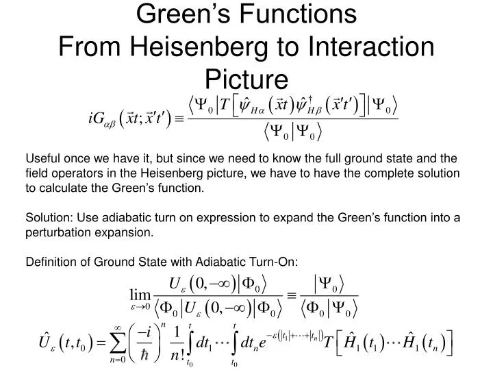
Green’s Functions From Heisenberg to Interaction Picture

1. Green’s FunctionsFrom Heisenberg to Interaction Picture Useful once we have it, but since we need to know the full ground state and the field operators in the Heisenberg picture, we have to have the complete solution to calculate the Green’s function. Solution: Use adiabatic turn on expression to expand the Green’s function into a perturbation expansion. Definition of Ground State with Adiabatic Turn-On:

2. Denominator Look at a general case: Denominator

3. Numerator F&W 6.31

4. Ratio Numerator operator (ignore denominator for now…it’s still there, but we’ll come back to it later: Explicitly time ordered product of all operators

5. Numerator (continued) Break up original sum to group with n ti’s > t and m n ti’s < t See F&W, p. 84 Use delta function to eliminate ν sum. (Note: there my be a -1 from T product.)

6. Conclusion Corollaries

7. Green’s Function in terms of Fields

8. Green’s Function – First Term Evaluate for “Free Fermion” Model in interaction picture: Break up c’s: Destroys particles Creates holes

9. First Term (continued) For Excited Electron Energy Ground State Energy Energy Missing Because of Holes

10. First Term (continued) For 0 0 You get b’s with a minus sign from reversing operators For Thus: Hole Part Electron part

11. Generalized Particles and Holes Like a’s – annihilate ground state Like b’s – does not annihilate ground state Can write products in terms of these

12. Two Types of Products Time Ordered Product – Put lower times to right. Normal Ordered Product – Put annihilation operators on right. Important property of Normal Ordered Product

13. Contractions Define Contractions as: Should be like (anti)commutator or zero. Most are zero. +(-) bosons(fermions) (anti) commutation

14. Non-Zero Contractions 0 0

15. Wick’s Theorem Appropriate sign is sign you get when you bring the two operators next to each other. 6 operators 15 contractions (9 are zero) 6 non-zero contraction

16. First Order Green’s Function (A) (B) (C) (D) (E) (F)

17. Diagram Analysis Propogator Term Potential Term

18. Six Diagrams for G1 (C) (A) (B) Disconnected Disconnected (E) (F) (D) Equivalent to (C) Equivalent to (D)

19. Meaning of G(x,x) Comes from potential terms contracting with themselves. Propagator interacting with background field Have to be very careful relativistically here!

20. Factor Out Disconnected Graphs OK to do to a given order in perturbation theory 1 This part is what you get from denominator: Hence, denominator cancels it out!!!

21. Multiple Integrals Graphs differ by dummy variables of integration. Integrals are the same. The multiplicity cancels out the 1/n! in front.

22. Feymann Rules • Draw all topologically distinct connected diagrams with n intersection lines U and 2n+1 directed Green’s functions G0. • Label each vertex with a four-dimensional space-time point x. • Each solid line represents a Green’s function G0αβ(x,y) running from y to x. • Each wavy line represents an interaction U(x,y)=V(x,y)δ(tx-ty) • Integrate all internal variables over space and time. • There is a spin product along each continuous fermion line including the potentials at the vertex. • Affix a sign factor of (-1)F to each term where F is the number of closed fermion loops in the diagram. • To compute G(x,y) assign a factor of (i/hbar)^n to each nth order term. • Interpret the equal time Green’s function as G(xt,xt+).