Download
1 / 18
470 likes | 1.13k Views
Inverting Magnetic Anomalies with UBC-IAG’s MAG3D and Using Images from SURFER and VOXLER. INVERSIONS AND CONSTRAINTS INVERSION Find a 3D subsurface distribution of physical properties that explains geophysical observations The results are not unique; many solutions are possible

E N D
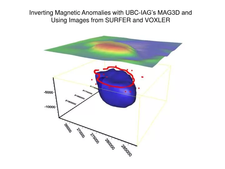
Inverting Magnetic Anomalies with UBC-IAG’s MAG3D andUsing Images from SURFER and VOXLER
INVERSIONS AND CONSTRAINTS • INVERSION • Find a 3D subsurface distribution of physical properties that explains geophysical observations • The results are not unique; many solutions are possible • Finding a solution is simple but you want an accurate and realistic solution • ADD CONSTRAINTS • Impose limits or conditions on the inversions • The calculated model must be consistent with geophysical observations as well as be geologically reasonable • Examples: • Geological observations • Smoothness • Depth weighting
Inverse & Constraints - Example The answer is 4 What is the Question? • Possibilities: • -1+5, 2.5+1.5, 6-2, -8.5+12.5 … this could go on forever • Constraint = positive numbers • 1.5 + 2.5, 2 + 2, 0.5 + 3.5, … still infinite • Constraint = positive integers • 1 + 3, 2 + 2, 3 + 1, which do we choose? • Constraint = minimum length • ||m||2 • 1+3: 12+32 = 1+9 = 10 • 2+2: 22+22 = 4+4 = 8 • 3+1: 32+12 = 9+1 = 10 • With these constraints, the solution is 2 +2
From: http://www.eos.ubc.ca/ubcgif/ Obtaining the IAG resource package – the educational license version is free! The package is distributed via flintbox , a global intellectual property exchange. You will need a high speed internet connection, a current browser (Microsoft I.E. or Mozilla Firefox are recommended), and at least 150Mbytes of free space on a computer running a Windows XX operating system. Download the IAG resource package for no charge from http://www.flintbox.com/technology.asp?Page=2732, or search for “IAG” at www.flintbox.com. You will be required to sign up for a free basic user account, read and agree to the license agreement, and download the 87 Mbyte installation executable file. These free versions of the codes are fully functional except that the number of data points (200), and the size (number of cells < 12,000) of models are both restricted
MAG3D is the code of interest for the Applied Magnetics class. MAG3D is a program library for carrying out forward modeling and inversion of surface, airborne, and/or borehole magnetic data in three dimensions. Updated to Version 4.0 June 2005. • Reading Chapter 1 of the MAG3D manual provides insight into the inversion techniques and assumptions: • http://www.eos.ubc.ca/ubcgif/iag/sftwrdocs/mag3d/background.htm • Chapter 1 of the MAG3D manual: b. Forward Modeling c. Inversion Methodology d. Depth Weighting e. Wavelet Compression of Sensitivity f. Choice of Tradeoff Parameter g. Example of Inversion h. References • The FAQ page, as with others pages in the manuals, provides relevant information: • http://www.eos.ubc.ca/ubcgif/iag/sftwrdocs/technotes/faq.htm
Steps in inverting a magnetic anomaly with the UBC-IAG inverse programs: • Determine and isolate the anomaly of interest; avoid anomalies at the edge of your grids • Remove a regional field if necessary. The more isolated an anomaly is the better the results
Choose and isolate an anomaly using Surfer’s “grid extract” tool
Choose and isolate an anomaly using Surfer’s “grid extract” tool Next we remove a planar regional and subtract the midrange from the grid to center the values around zero nanotesla.
We have some interfering anomalies and a few smaller sources surrounding the anomaly of interest. Next, we have to get the observed field data into the format necessary for UBC-IAG’s software. To do so: In Surfer’s “grid node editor”, save the grid as an ASCII.dat file
The data file format, shown below, for data in western Montana would be something like: 68 14 5600068 14 1666E1 N1 Elev1 TMI1 Err1E2 N2 Elev2 TMI2 Err2 … …E666 N666 Elev666 TMI666 Err666 Where idat signifies “1 component data” and Err666 is the error associated with the observation. You should calculate the error as a minimum positive number added to a percent of the TMI value (e=fabs(.1*d+10)). Errors must be positive and reasonably large. If you only use a percent, then the error for observations near zero nt will be near zero and the inversion will not finish (nor tell you why…).
Formatted data – calculate error column with: e=fabs(.1*d+10) This file works.
“gm-data-viewer.exe” will let you see the data and downsample the number of observations to a reasonable value. Often it is best to run the first inversions on a limited data set while you experiment with parameters and evaluate results. The educational version only allows 200 data points and 12,000 cells.
Starting the GUI:mag3d-gui.exeyields the screen to the right where you proceed to: • Browse to your data file (less than 201 points) • Create a mesh (less than 12,000 cells) & save it as ___.msh • File/Save the parameters • RUN and see if it works. The *.log files give little hints to possible errors
Next, run MeshTools3d.exe and open the [maginv3d.sus] which is what MAG3D writes for a result. Under “options” set the range for susceptibilities of interest and remove padding cells to enhance the display.
The limitations of the educational version cut into the quality of the result for this region. But, you can do well with smaller, single anomalies.
Using the commercial version with much smaller cells results in a substantial improvement for visualization
UBC_IAG provides “model2xyz.exe” which puts the model coordinates into a file compatible with Golden Software’s VOXLER 3D visualization software
Here, magenta dots show the maxima of the horizontal gradient of the pseudogravity calculated from the TMI (relief map) shown above two isosurfaces from the inverse model