Download
1 / 24
240 likes | 263 Views
Relative-timing based verification of timed circuits and systems . Hoshik Kim and Peter A. Beerel Department of EE-Systems University of Southern California IWLS ’99 June 27-30, 1999. Motivation: Timed Circuits and Systems. Definition

E N D
Relative-timing based verification of timed circuits and systems Hoshik Kim and Peter A. Beerel Department of EE-Systems University of Southern California IWLS ’99 June 27-30, 1999
Motivation: Timed Circuits and Systems Definition • Any circuit/specification in which timing constraints/assumptions are necessary to ensure “correct” operation Examples • Delayed-reset Domino [Nowka et al., ICCD98] • Self-Resetting Domino [Chappell et al., IBM96] • Timed (asynchronous) circuits [Intel’s RAPPID, ASYNC99] Advantages • Extremely fast and dense Disadvantages • Hard to design and verify • Requires complicated timing verification
Self-Resetting Domino (SRCMOS) Characteristics • The input signal to a SRCMOS stage is a pulserather than a level Input pulse requirements • must last until after N1 falls • must be lessthan theresetdelay (green path) Key implication • Thus, atwo-sided constrainton the pulse width exists N2 Q N1 B A A self-resetting 2-input OR gate
Timed Circuits • Each circuit node • is a state variable Asynchronous Reachability Analysis Static Timing Analysis • Very powerful • More computationally expensive • Well-known and fast • Does not easily handle two-sided constraints Possible Verification Approaches • Our approach: Reduce the cost of asynchronous analysis
000000 A A+ B+ u1 B 010000 100000 [0.2, 4] 110000 u2 C u + 1 State = [A B C u u u ] 1 2 3 110100 [0.3, 3] [0.2, 4] [2, 4] [1, 5] C+ u3 111100 u + + = u + 2 3 A-,B- [0.2, 4] 111110 111101 A- B- B- Specification 101101 u - Circuit [1, 5] [2, 4] 3 Timed State Space F Current State-of-the-Art: Explicit-timing Features [Belluomini et al., ASYNC99] • Bounds of delays used • Time is dense -> timed state space is infinite! • Timed state space representation • States labeled with binary value of all signals • Regions used to characterize the time in each state
Issues with Explicit-timing approach • Explicit-timing verification must overcome double exponential complexity(state space+timing) • Timing margins may need to be overly conservative • Delay bounds must be valid across process variations • Minor design changes that affect bounds require complete re-verification
A B x y Relative-Timing (RT) Verification Verification methodology • Find relative-timing constraints on path delays that guarantee correctness • If red path delay is smaller than green path, y is stable high -> OK • If red path delay is larger than yellow path, y has neg. pulse -> OK • Otherwise, a runt pulse (or hazard) can occur -> FAILURE • Analyze post-layout circuits to validate constraints • SPICE-level simulation OR • Simpler timing analysis using bounded delays
Advantages of Relative-Timing (RT) • Reduces verification complexity • RT techniques do not need to model timers • Reduces complexity exponentially • Facilitates use of mature symbolic methods • Facilitates tighter timing margins • RT constraints can be verified very aggressively • Promotes easy incremental verification • Many minor design changes easily verifiable (e.g., simulation) • E.g., transistor sizing, layout, technology/process migration
A B x y The problem statement Definitions • Event chain • Sequence of transitions along a circuit path • Delay of an event chain • associated path delay • E.g., DB+A-y- = DB+A- + DA-y- • Relative-timing constraint • Ordered triple of event chain delays • view as two sided constraint on a target event chain delay • E.g., DB+A-< DB+x+ < DB+A-y- Our Goal • Find relative-timing constraints necessary and sufficient for correctness
Our approach Step 1 • Perform asynchronous reachability analysis (w/o regions) • States labeled with binary values of all signals • Over approximation because time is not considered Step 2 • Identify all possible failure transitions • Formalized with notion of an “event triples” Step 3 • Determine causality of events in event triple • Formalized with notion of an “event PN” Step 4 • Find relative timing constraint for each event PN • Formalized with notion of “time separation of events (TSE)” [Xie et al., ASYNC99]
l1 l2 t Fail u1 t u1 t t u2 u2 Q(t) Reachability Graph (from Step 1) Event Triples Target event t • labels a failure transition (causes a race) Dangerous set of states • Q(t) = {s | }; Event triple (l, t, u) • tis atarget event • lis a lower bound event which entersQ(t) • uis an upperbound event which escapesQ(t) Interpretation • Target failure occurs if t happens after l enters Q(t) but before u occurs
Event triple (l, t, u) Synchronization events t s1 Event PN l u s2 An Event PN The Goal • Characterize the causality of events in an event triple Event PN • An acyclic Petri net describing causality of events Our Approach • Create an Event PN to capture the causality • Find a constraint using TSE’s. • {TSE (l, t) > 0} ^ {TSE (t, u) > 0} • TSE expressions relate to delays of gates along circuit paths
Untimed analysis to find out event triples One possible approach • Leverage off of advanced verification techniques [Pastor99, Vakilotojar98, Yoneda96, Yenigun99] • Mapping PN from ETSiscomputationally complex • The assignments of delays to places is unclearwhen label splitting occurs Circuit Description Specification Transition System (TS) Elementary TS (ETS) [Cortadella et al.95] Event PN for each event triple RT constraints
Untimed analysis to find out event triples Petri net model of the circuit Gates Library (Petri net models) Event PN for each event triple An alternative approach • Creating the Petri net model of a circuit is straight forward • Leverage off of advanced verification techniques [Pastor99, Vakilotojar98, Yoneda96, Yenigun99] • The correspondence of delays on places and gate delays is pre-determined in the Petri net gate library • Looks more promising Circuit Description Specification RT constraints
000000 000 A+ B+ A+ B+ 010000 100000 010 100 110000 u + 1 State = [A B C u u u ] 1 2 3 C- 110100 110 C+ State = [A B C] C+ 111100 u + u + 2 3 111 A-,B- 111110 111101 A- B- A- B- B- 101101 A- 011110 111111 u - u - 3 101 2 011 Specification 101100 1011111 011100 011111 A- B- B- A 001 001111 101110 011101 u1 B A- 001110 001101 u - 1 F 001100 C- C u2 A- 101001 A- 011010 u - u - u + 3 2 u + 2 3 101000 011011 101011 011000 B- A- u3 101010 001011 011001 001010 001001 001000 Sum-of-Products C-element Reachability Graph Example 1: Static C-element
000000 A+ B+ 010000 100000 110000 u + 1 State = [A B C u u u ] 1 2 3 110100 C+ 111100 u + u + 2 3 A-, B- 111110 111101 A- B- B- 101101 A- 011110 111111 u - u - 3 2 101100 1011111 011100 011111 A- B- B- 001111 101110 011101 A-/1 001110 001101 u - 1 F 001100 C- B- A- B- 101001 A- 011010 u - u - u + 3 2 u + 2 3 101000 011011 101011 011000 B- A- 101010 001011 011001 001010 001001 001000 Reachability Graph Example 1 (cont.) • Generate RT Constraints: 1. T = {B-, A-} 2. For t = B-, L = {C+}, U = {u3+} 3. Find an event PN and thus RT constraint for event triple (C+, B-, u3+) 4. For t = A-, L = {C+}, U = {u2+} 5. Repeat Step 3 for event triple (C+, A-, u2+) • The circuit will work “correctly” unless it satisfies any of the RT constraints.
AND2 Specification A u1 AND2 B u2 C u3 OR3 Circuit AND2 Example 1 (cont.) A partial marking corresponds to a dangerous states set Q “?” indicates “input” “!” indicates “output”
Example 1 (cont.) • Event PN for event triple (C+, B-, u3+) • Double synchronization events here • Thus,only upper and lower bounds on TSE can be found [Xie et al.99] • The upper bound of TSE (TSEu) will be used in the constraints to beconservative • Event triple (l, t, u) = (C+, B-, u3+) • TSE (C+, B-) = d(p3) > 0 (Delay of a place is always positive) • Leads to a trivial two-sided constraints • TSEu (B-, u3+) = • max [max {d(p4) + d(p2) + d(p5), d(p6)} - {d(p4) + d(p2) + d(p3)}, d(p5) - d(p3)] > 0 • {DB+u1+C+B- < max (DB+u1+C+u3+, DB+u3+)} {DC+B- < DC+u3+}
A y x B C C Circuit Example 2: Two-sided constraints 000 00000 A+ A+ 100 10000 B+ y+ State = [A B C] B+ 11000 10001 C- y+ x+ B+ 110 C- C+ A- 11001 11010 y+ x+ State= [A B C x y] 010 111 11011 C+ A- C+ A- A- 11111 011 F A- B- A- 001 x+ A- 00100 01000 y- x+ Specification y- 00101 01010 01001 y+ x- 00111 C+ 01011 B- 01111 Reachability Graph
00000 A+ 10000 B+ y+ 11000 10001 C- y+ x+ B+ 11001 11010 y+ x+ State = [A B C x y] 11011 C+ A- A- 11111 F A- A- x+ A- 00100 01000 y- x+ y- 00101 01010 01001 y+ x- 00111 C+ 01011 B- 01111 Reachability Graph Example 2 (cont.) • Generate Chain Constraints : 1. T = {A-, x+} 2. For t = A-, L = {B+}, U = {x+, y+} 3. Find an event PN and sub-constraint for each event triple (B+, A-, x+) and (B+, A-, y+). Conjunction of all sub-constraints is an RT constraint 4. For t = x+, L = {A-}, U = {y-} 5. Repeat Step 3 for event triple (A-, x+, y-)
OR2 Specification A y x B C C Buffer C-element Circuit Example 2 (cont.) A partial marking corresponds to a dangerous states set Q “?” indicates “input” “!” indicates “output”
Example 2 (cont.) • Event PN for event triple (A-, x+, y-) 00000 A+ 10000 B+ y+ 11000 10001 C- y+ x+ B+ 11001 11010 y+ x+ State = [A B C x y] 11011 C+ A- A- 11111 F A- • Event triple(l, t, u) = (A-, x+, y-) • TSE (A-, x+) = d(p1) - d(p2) > 0 • TSE (x+, y-) = {d(p2) + d(p3)} - d(p1) > 0 • (DB+A- < DB+x+)^(DB+x+ < DB+A-y-) • \ DB+A- < DB+x+ < DB+A-y- • If we had only one bound DB+x+ < DB+A-y-, we would remove good states -> false negatives A- x+ A- 00100 01000 y- x+ y- 00101 01010 01001 y+ x- 00111 C+ 01011 B- 01111
Conclusion • We presented novel verification techniques to support emerging high performance circuit design techniques. • These techniques identify a set of two-sided path delay constraints that are sufficient to find any failure of the circuits • Constraints can be verified using simulation or simpler timing analysis
Future Work • Refine and implement the theory and algorithm • Combine with hierarchical and other partial order approaches • Test on both aggressively designed synchronous and asynchronous circuits