Download
1 / 26
310 likes | 1.24k Views
Stationarity, Non Stationarity, Unit Roots and Spurious Regression. Roger Perman Applied Econometrics Lecture 11. Stationary Time Series. Exhibits mean reversion in that it fluctuates around a constant long run mean Has a finite variance that is time invariant

E N D
Stationarity, Non Stationarity, Unit Roots and Spurious Regression Roger Perman Applied Econometrics Lecture 11
Stationary Time Series Exhibits mean reversion in that it fluctuates around a constant long run mean Has a finite variance that is time invariant Has a theoretical covariance between values of ytthat depends only on the difference apart in time
Stationary time series WHITE NOISE PROCESS Xt = ut ut ~ IID(0, σ2 )
Many Economic Series Do not Conform to the Assumptions of Classical Econometric Theory Share Prices Exchange Rate Income
Non Stationary Time Series There is no long-run mean to which the series returns and/or The variance is time dependent and goes to infinity as time approaches to infinity Theoretical autocorrelations do not decay but, in finite samples, the sample correlogram dies out slowly The results of classical econometric theory are derived under the assumption that variables of concern are stationary. Standard techniques are largely invalid where data is non-stationary
Non-stationary time series UK GDP (Yt) The level of GDP (Y) is not constant and the mean increases over time. Hence the level of GDP is an example of a non-stationary time series.
Non-stationary time series RANDOM WALK Xt = Xt-1 + utut ~ IID(0, σ2 ) Mean: E(Xt) = E(Xt-1) (mean is constant in t) X1 = X0+ u1(take initial value X0) X2 = X1 + u2 = (X0 + u1 ) + u2 … Xt = X0 + u1 + u2 +…+ ut E(Xt) = E(X0 + u1 + u2 +…+ ut)(take expectations) = E(X0)= constant
Non-stationary time series RANDOM WALK Xt = Xt-1 + utut ~ IID(0, σ2 ) Xt = X0 + u1 + u2 +…+ ut Variance: Var(Xt) = Var(X0) + Var(u1) +…+ Var(ut) = 0 + σ2 +…+ σ2 = t σ2 (variance is not constant through time)
Non-stationary time series: Random WalkXt = Xt-1 + utut ~ IID(0, σ2 )
Constant covariance - use of correlogram Covariance between two values of Xt depends only on the difference apart in time for stationary series. Cov(Xt ,Xt+k) = χ(k)(covariance is constant in t) (A) Correlation for 1980 and 1985 is the same as for 1990 and 1995. (i.e. t = 1980 and 1990, k = 5) (B) Correlation for 1980 and 1987 is the same as for 1990 and 1997. (i.e. t = 1980 and 1990, k = 7)
Non-stationary time series UK GDP (Yt) - correlogram For non-stationary series the Autocorrelation Function (ACF) declines towards zero at a slow rate as k increases.
Stationary time series First difference of GDP is stationary ΔYt =Yt -Yt-1 - Growth rate is reasonably constant through time. Variance is also reasonably constant through time
Stationary time series UK GDP Growth (Δ Yt) - correlogram Sample autocorrelations decline towards zero as k increases. Decline is rapid for stationary series.
Non-stationary Time Series: summary Relationship between stationary and non-stationary process AutoRegressive AR(1) process Xt = α + ρXt-1 + ut ut ~ IID(0, σ2 ) ρ < 1 stationary process - “process forgets past” ρ = 1 non-stationary process - “process does not forget past” α = 0 without drift α 0 with drift
Stationary time series with driftXt = α + 0.5*Xt-1 + utut ~ IID(0, σ2 )
Non-stationary time series: Random Walk with DriftXt = α + Xt-1 + utut ~ IID(0, σ2 )
Time Series Models: summary General Models AutoRegressive AR(1) process without drift Xt = ρXt-1 + ut ρ < 1 stationary process - “process forgets past” ρ = 1 non-stationary process - “process does not forget past” AutoRegressive AR(k) process without drift Xt = ρ1Xt-1 + ρ2Xt-2 + ρ3Xt-3 + ρ4Xt-4 +…+ ρkXt-k + ut
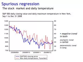
Spurious Regression Problem yt = yt-1 + ut ut ~ iid(0,σ2) xt = xt-1 + vt vt ~ iid(0,σ2) utandvtare serially and mutually uncorrelated yt = β0 + β1xt + εt since yt and xtare uncorrelated random walks we should expect R2 to tend to zero. However this is not the case. Yule (1926): spurious correlation can persist in large samples with non-stationary time series. - if two series are growing over time, they can be correlated even if the increments in each series are uncorrelated
Spurious Regression Problem Two random walks generated from Excel using RAND() command hence independent yt = yt-1 + ut ut ~ iid(0,σ2) xt = xt-1 + vt vt ~ iid(0,σ2)
Spurious Regression Problem Plot Correlogram using PcGive (Tools, Graphics, choose graph, Time series ACF, Autocorrelation Function) yt = yt-1 + ut ut ~ iid(0,σ2) xt = xt-1 + vt vt ~ iid(0,σ2)
Spurious Regression Problem Estimate regression using OLS in PcGive yt = β0 + β1xt + εt based on two random walks yt = yt-1 + ut ut ~ iid(0,σ2) xt = xt-1 + vt vt ~ iid(0,σ2) EQ( 1) Modelling RW1 by OLS (using lecture 2a.in7) The estimation sample is: 1 to 498 Coefficient t-value Constant 3.147 25.8 RW2 -0.302 -15.5 sigma 1.522 RSS 1148.534 R^2 0.325 F(1,496) = 239.3 [0.000]** log-likelihood -914.706 DW 0.0411 no. of observations 498 no. of parameters 2
Trend: Deterministic or Stochastic? The First The Second (with a2 <1 and a3 >0)
This series has a deterministic trend (if a3 > 0) Classical inference is valid (provided that a2is less than 1). The series is transformed to a stationary series by subtracting the deterministic trend from the left side (and so the right side).
This series is non-stationary - the trend is stochastic Classical inference is not valid The series is called “difference stationary” Random Walk With Drift
Types of Model from the General Formulation Parameter Set Description Properties 1 Deterministic Trend With m ¹ f < b ¹ 0 , 1 , 0 1 Stationary AR(1) components m ¹ f = b ¹ Random Walk with Drift and 2 0 , 1 , 0 I (1) 1 Deterministic Trend m ¹ f = b = 3 Random Walk with Drift 0 , 1 , 0 I I (0) (1) 1 m ¹ f = b ¹ 4 Deterministic Trend 0 , 0 , 0 I (0) 1 m = f = b = Pure Random Walk 5 0 , 1 , 0 I (1) 1