Download
1 / 91
910 likes | 913 Views
This text explains the standard methodology for evaluating machine learning models using labeled datasets, N-fold cross-validation, and tuning sets. It highlights the importance of proper experimental methodology and the impact it can have on accuracy. The text also discusses parameter setting, using multiple tuning sets, and the use of test sets to estimate future performance.

E N D
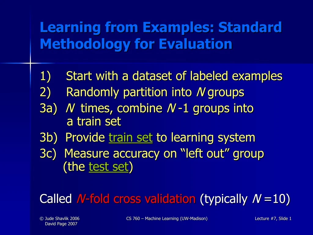
Learning from Examples: Standard Methodology for Evaluation 1) Start with a dataset of labeled examples 2) Randomly partition into N groups 3a) N times, combine N -1 groups into a train set 3b) Provide train set to learning system 3c) Measure accuracy on “left out” group (the test set) CalledN-fold cross validation(typically N =10) CS 760 – Machine Learning (UW-Madison)
Using Tuning Sets • Often, an ML system has to choose when to stop learning, select among alternative answers, etc. • One wants the model that produces the highest accuracy on future examples (“overfitting avoidance”) • It is a “cheat” to look at the test set while still learning • Better method • Set aside part of the training set • Measure performance on this “tuning” data to estimate future performance for a given set of parameters • Use best parameter settings, train with all training data (except test set) to estimate future performance on new examples CS 760 – Machine Learning (UW-Madison)
Experimental Methodology: A Pictorial Overview collection of classified examples testing examples training examples Statistical techniques such as 10-fold cross validation and t-tests are used to get meaningful results tune set train’ set classifier generate solutions select best expected accuracy on future examples LEARNER CS 760 – Machine Learning (UW-Madison)
Proper Experimental Methodology Can Have a Huge Impact! A 2002 paper in Nature (a major, major journal) needed to be corrected due to “training on the testing set” Original report : 95% accuracy (5% error rate) Corrected report (which still is buggy): 73% accuracy (27% error rate) Error rate increased over 400%!!! CS 760 – Machine Learning (UW-Madison)
Parameter Setting Notice that each train/test fold may get different parameter settings! • That’s fine (and proper) I.e. , a “parameterless”* algorithm internally sets parameters for each data set it gets CS 760 – Machine Learning (UW-Madison)
Using Multiple Tuning Sets • Using a single tuning set can be unreliable predictor, plus some data “wasted”Hence, often the following is done: 1) For each possible set of parameters, a) Divide training data into train’ and tune sets, usingN-fold cross validation b) Score this set of parameter value, average tune set accuracy 2) Use best set of parameter settings and all (train’ + tune) examples 3) Apply resulting model to test set CS 760 – Machine Learning (UW-Madison)
K=0 tune train Tuning a Parameter- Sample Usage Step1: Try various values for k (eg, # of hidden units). Use 10 train/tune splits for each k Step2: Pick best value for k (eg. k = 2), Then train using all training data Step3: Measure accuracy on test set 1 2 Tune set accuracy (ave. over 10 runs)=92% 10 1 K=2 Tune set accuracy (ave. over 10 runs)=97% 2 10 … 1 Tune set accuracy (ave. over 10 runs)=80% K=100 2 10 CS 760 – Machine Learning (UW-Madison)
What to Do for the FIELDED System? • Do not use any test sets • Instead only use tuning sets to determine good parameters • Test sets used to estimate future performance • You can report this estimate to your “customer,” then use all the data to retrain a “product” to give them CS 760 – Machine Learning (UW-Madison)
What’s Wrong with This? • Do a cross-validation study to set parameters • Do another cross-validation study, using the best parameters, to estimate future accuracy • How will this relate to the “true” future accuracy? • Likely to be an overestimate What about • Do a proper train/tune/test experiment • Improve your algorithm; goto 1 (Machine Learning’s “dirty little” secret!) CS 760 – Machine Learning (UW-Madison)
Why Not Learn After Each Test Example? • In “production mode,” this would make sense (assuming one received the correct label) • In “experiments,” we wish to estimate Probability we’ll label the next example correctly need several samples to accurately estimate CS 760 – Machine Learning (UW-Madison)
# of Examples < 50 50 < ex’s < 100 > 100 Method Instead, use Bootstrapping (B. Ephron) See “bagging” later in cs760 Leave-one-out (“Jack knife”) N = size of data set (leave out one example each time) 10-fold cross validation (CV),also useful for t-tests Choosing a Good Nfor CV(from Weiss & Kulikowski Textbook) CS 760 – Machine Learning (UW-Madison)
Fold 1 Recap: N-fold Cross Validation • Can be used to 1) estimate future accuracy (by test sets) 2)choose parameter settings (by tuning sets) • Method 1) Randomly permute examples 2) Divide into Nbins 3) Train on N-1 bins, measure performance on bin ”left out” 4) Compute average accuracy on held-out sets Examples Fold 5 Fold 2 Fold 3 Fold 4 CS 760 – Machine Learning (UW-Madison)
Confusion Matrices- Useful Way to Report TESTSET Errors Useful for NETtalk testbed – task of pronouncing written words CS 760 – Machine Learning (UW-Madison)
Scatter Plots- Compare Two Algo’s on Many Datasets Each dot is the error rate of the two algo’s on ONE dataset Algo A’s Error Rate Algo B’s Error Rate CS 760 – Machine Learning (UW-Madison)
Statistical Analysis of Sampling Effects • Assume we get e errors on Ntest set examples • What can we say about the accuracy of our estimate of the true (future) error rate? • We’ll assume test set/future examples independently drawn (iid assumption) • Can give probability our true error rate is in some range – error bars CS 760 – Machine Learning (UW-Madison)
The Binomial Distribution • Distribution over the number of successes in a fixed number n of independent trials (with same probability of success p in each) CS 760 – Machine Learning (UW-Madison)
Using the Binomial • Let each test case (test data point) be a trial, and let a success be an incorrect prediction • Maximum likelihood estimate of probability p of success is fraction of predictions wrong • Can exactly compute probability that error rate estimate p is off by more than some amount, say 0.025, in either direction • For large N, this computation’s expensive CS 760 – Machine Learning (UW-Madison)
Central Limit Theorem • Roughly, for large enough N, all distributions look Gaussian when summing/averaging N values 0 1 Ave Y over Ntrials (repeated many times) Surprisingly, N = 30 is large enough! (in most cases at least) - see pg 132 of textbook CS 760 – Machine Learning (UW-Madison)
Confidence Intervals CS 760 – Machine Learning (UW-Madison)
As You Already Learned in “Stat 101” If we estimate μ (mean error rate)and σ (std dev), we can say our ML algo’s error rate is μ± ZMσ ZM : value you looked up in a table of N(0,1) for desired confidence; e.g., for 95% confidence it’s 1.96 CS 760 – Machine Learning (UW-Madison)
The Remaining Details CS 760 – Machine Learning (UW-Madison)
Alg 1 vs. Alg 2 • Alg 1 has accuracy 80%, Alg 2 82% • Is this difference significant? • Depends on how many test cases these estimates are based on • The test we do depends on how we arrived at these estimates CS 760 – Machine Learning (UW-Madison)
Leave-One-Out: Sign Test • Suppose we ran leave-one-out cross-validation on a data set of 100 cases • Divide the cases into (1) Alg 1 won, (2) Alg 2 won, (3) Ties (both wrong or both right); Throw out the ties • Suppose 10 ties and 50 wins for Alg 1 • Ask: Under (null) binomial(90,0.5), what is prob of 50+ or 40- successes? CS 760 – Machine Learning (UW-Madison)
What about 10-fold? • Difficult to get significance from sign test of 10 cases • We’re throwing out the numbers (accuracy estimates) for each fold, and just asking which is larger • Use the numbers… t-test… designed to test for a difference of means CS 760 – Machine Learning (UW-Madison)
Paired Student t-tests • Given • 10 training/test sets • 2 ML algorithms • Results of the 2 ML algo’s on the 10 test-sets • Determine • Which algorithm is better on this problem? • Is the difference statistically significant? CS 760 – Machine Learning (UW-Madison)
Paired Student t–Tests (cont.) Example Accuracies on Testsets Algorithm 1: 80% 50 75 … 99 Algorithm 2: 79 49 74 … 98 • : +1 +1 +1 … +1 • Algorithm 1’s mean is better, but the two std. Deviations will clearly overlap • But algorithm1 is always better than algorithm 2 i CS 760 – Machine Learning (UW-Madison)
The Random Variable in the t-Test Consider random variable • = Algo A’s Algo B’s test-seti minus test-seti error error i • Notice we’re “factoring out” test-set difficulty by looking at • relative performance • In general, one tries to explain variance • in results across experiments • Here we’re saying that • Variance = f(Problem difficulty) + g(Algorithm strength) CS 760 – Machine Learning (UW-Madison)
More on the Paired t-Test Our NULLHYPOTHESIS is that the two ML algorithms have equivalent average accuracies • i.e. differences (in the scores) are due to the “random fluctuations” about the mean of zero We compute the probability that the observed δ arose from the null hypothesis • If this probability is low we rejectthe null hypo and say that the two algo’s appear different • ‘Low’ is usually taken as prob ≤ 0.05 CS 760 – Machine Learning (UW-Madison)
P(δ) The Null Hypothesis Graphically (View #1) 1. Assumezero mean and use the sample’s variance(sample = experiment) δ Does our measured δ lie in the regions indicated by arrows? If so, reject null hypothesis, since it is unlikely we’d get such a δ by chance ½ (1 – M ) probability mass in each tail (ie, M inside)Typically M = 0.95 CS 760 – Machine Learning (UW-Madison)
P(δ) View #2 – The Confidence Interval for δ 2. Use sample’s mean and variance δ Is zero in the M % of probability mass?If NOT, reject null hypothesis CS 760 – Machine Learning (UW-Madison)
The t-test Confidence Interval • Given:δ1 , … , δN where where each δi is measured on a test set of at least 30* examples (so the “Central Limit Theorem” applies for individual measurements) • Compute: Confidence interval, Δ, at the M % level for the mean difference See if contains ZERO. If not, we can reject the NULL HYPOTHESIS i.e. algorithms A & B perform equivalently * Hence if Nis the typical 10, our dataset must have ≥ 300 examples CS 760 – Machine Learning (UW-Madison)
The t-Test Calculation We don’t know an analytical expression for the variance, so we need to estimate it on the data Compute • Mean • Sample Variance • Lookupt value for N folds and Mconfidence level - “N-1” is called the degrees of freedom - As N∞, tM,N-1 and ZM equivalent See table 5.6 in Mitchell CS 760 – Machine Learning (UW-Madison)
The t-test Calculation (cont.)- Using View #2 (get same result using view #1) Calculate The interval contains 0 if PDF δ CS 760 – Machine Learning (UW-Madison)
Some Jargon: P–values(Uses View #1) P-Value = Probability of getting one’s results or greater, given the NULL HYPOTHESIS (We usually want P ≤ 0.05 tobe confident that a difference is statistically significant) NULL HYPO DISTRIBUTION P CS 760 – Machine Learning (UW-Madison)
From Wikipedia(http://en.wikipedia.org/wiki/P-value) The p-value of an observed value Xobserved of some random variable Xis the probability that, given that the null hypothesis is true, X will assume a value as or more unfavorable to the null hypothesis as the observed value Xobserved "More unfavorable to the null hypothesis" can in some cases mean greater than, in some cases less than, and in some cases further away from a specified center CS 760 – Machine Learning (UW-Madison)
“Accepting” the Null Hypothesis Note: even if the p–value is high, we cannot assume the null hypothesis is true Eg, if we flip a coin twice and get one head, can we statistically infer the coin is fair? Vs. if we flip a coin 100 times and observe 10 heads, we can statistically infer coin is unfair because that is very unlikely to happen with a fair coin How would we show a coin is fair? CS 760 – Machine Learning (UW-Madison)
More on the t-Distribution We typically don’t have enoughfolds to assume the central-limit theorem. (i.e. N < 30) • So, we need to use the t distribution • It’s wider (and hence, shorter) than the Gaussian (Z) distribution (since PDFs integrate to 1) • Hence, our confidence intervals will be wider • Fortunately, t-tables exist Gaussian tN different curve for each N CS 760 – Machine Learning (UW-Madison)
Some Assumptions Underlying our Calculations • General • Central Limit Theorem applies (I.e., >= 30 measurements averaged) • ML-Specific • #errors/#tests accurately estimates p, prob of error on 1 ex. • used in formula for s which characterizes expected future deviations about mean (p) • Using independent sample space of possible instances • - representative of future examples • - individual ex’s iid drawn • For paired t-tests, learned classifier same for each fold (“stability”) since combining results across folds CS 760 – Machine Learning (UW-Madison)
Stability Stability = how much the model an algorithm learns changes due to minor perturbations of the training set Paired t-test assumptions are a better match to stable algorithm Example: k-NN, higher the k, the more stable CS 760 – Machine Learning (UW-Madison)
More on Paired t-Test Assumption Ideally train on one data set and then do a 10-fold paired t-test What we should do: traintest1 … test10 What we usually do: train1test1 … train10test10 However, not enough data usually to do the ideal If we assume that train data is part of each paired experiment then we violate independence assumptions - each train set overlaps 90% with every other train set Learned model does not vary while we’re measuring its performance CS 760 – Machine Learning (UW-Madison)
The Great Debate(or one of them, at least) • Should you use a one-tailed or a two-tailed t-test? • A two-tailed test asks the question: Are algorithms A and B statistically different? • A one-tailed test asks the question: Is algorithm A statistically better than algorithm B? CS 760 – Machine Learning (UW-Madison)
One vs. Two-Tailed Graphically P(x) One-Tailed Test x 2.5% 2.5% 2.5% Two-Tailed Test CS 760 – Machine Learning (UW-Madison)
The Great Debate (More) • Which of these tests should you use when comparing your new algorithm to a state-of-the-art algorithm? • You should use two tailed, because by using it, you are saying there is a chance I am better and a chance I am worse • One tailed is saying, I know my algorithm is no worse, and therefore you are allowed a larger margin of error By being more confident, it is easier to show significance! See http://www.psychstat.missouristate.edu/introbook/sbk25m.htm CS 760 – Machine Learning (UW-Madison)
Two Sided vs. One Sided You need to very carefully think about the question you are asking Are we within x of the true error rate? Measured mean mean - x mean + x CS 760 – Machine Learning (UW-Madison)
Two Sided vs. One Sided How confident are we that ML System A’s accuracy is at least 85%? 85% CS 760 – Machine Learning (UW-Madison)
Two Sided vs. One Sided Is ML algorithm A no more accurate than algorithm B? A - B CS 760 – Machine Learning (UW-Madison)
Two Sided vs. One Sided Are ML algorithm A and B equivalently accurate? A - B CS 760 – Machine Learning (UW-Madison)
Contingency Tables True Answer + - + AlgorithmAnswer - Counts of occurrences CS 760 – Machine Learning (UW-Madison)
TPR and FPR True Positive Rate = n(1,1) / ( n(1,1) + n(0,1) )(TPR) = correctly categorized +’s / total positives P(algo outputs + | + is correct) False Positive Rate = n(1,0) / ( n(1,0) + n(0,0) )(FPR) = incorrectly categorized –’s / total neg’s P(algo outputs + | - is correct) Can similarly define False Negative Rate and True Negative RateSeehttp://en.wikipedia.org/wiki/Type_I_and_type_II_errors CS 760 – Machine Learning (UW-Madison)
ROC Curves • ROC: Receiver Operating Characteristics • Started during radar research during WWII • Judging algorithms on accuracy alone may not be good enough when getting a positive wrong costs more than getting a negative wrong (or vice versa) • Eg, medical tests for serious diseases • Eg, a movie-recommender (ala’ NetFlix) system CS 760 – Machine Learning (UW-Madison)