Download
1 / 20
220 likes | 328 Views
Christian Byrnes Institute of theoretical physics University of Heidelberg (ICG, University of Portsmouth) David Wands, Kazuya Koyama and Misao Sasaki Diagrams: arXiv:0705.4096, JCAP 0711:027, 2007; Trispectrum: astro-ph/0611075, Phys.Rev.D74:123519, 2006 work in progress.

E N D
Christian Byrnes Institute of theoretical physics University of Heidelberg (ICG, University of Portsmouth) David Wands, Kazuya Koyama and Misao Sasaki Diagrams: arXiv:0705.4096, JCAP 0711:027, 2007; Trispectrum: astro-ph/0611075, Phys.Rev.D74:123519, 2006 work in progress Primordial non-Gaussianity from inflation Kosmologietag, Bielefeld, 8th May 2008
Motivation • Lots of models of inflation, need to predict many observables • Non-Gaussianity, observations improving rapidly • Not just which parameterises bispectrum • ACT, Planck, can observe/constrain trispectrum • 2 observable parameters • What about higher order statistics? • Or loop corrections? • Do they modify the predictions? • Diagrammatic method • Calculates the n-point function of the primordial curvature perturbation, at tree or loop level • Separate universe approach • Valid for multiple fields and to all orders in slow-roll parameters
The primordial curvature perturbation Calculate using the formalism (valid on super horizon scales) Separate universe approach Efoldings where and is evaluated at Hubble-exit Field perturbations are nearly Gaussian at Hubble exit Curvature perturbation is not Gaussian Starobinsky `85; Sasaki & Stewart `96; Lyth & Rodriguez ’05 Maldacena ‘01; Seery & Lidsey ‘05; Seery, Lidsey & Sloth ‘06
Diagrams from Gaussian initial fields • Here for Fourier space, can also give for real space • Rule for n-point function, at r-th order, r=n-1 is tree level • Draw all distinct connected diagrams with n-external lines (solid) and r propagators (dashed) • Assign momenta to all lines • Assign the appropriate factor to each vertex and propagator • Integrate over undetermined loop momenta • Divide by numerical factor (1 for all tree level terms) • Add all distinct permutations of the diagrams
Explicit example of the rules For 3-point function at tree level After integrating the internal momentum and adding distinct permutations of the external momenta we find
Bispectrum and trispectrum CB, Sasaki & Wands, 2006; Seery & Lidsey, 2006
Observable parameters, bispectrum and trispectrum We define 3 k independent non-linearity parameters Note that and both appear at leading order in the trispectrum The coefficients have a different k dependence, The non-linearity parameters are
“Single” field inflation • Specialise to the case where one field generates the primordial curvature perturbation • Includes many of the cases considered in the literature: • Standard single field inflation • Curvaton scenario • Modulated reheating Only 2 independent parameters Consistency condition between bispectrum and 1 term of the trispectrum
Loop corrections The integrals need a cut off k – observed scale k max – smoothing scale L – IR cut off, large scales, L > 1/H Size of the loop contribution appears to depend on the cut off
Importance of the loop correction? What is L? For L~Horizon scale, loop correction to power spectrum is tiny For L~eternal inflation, loop correction dominates! Is it just a question of renormalisation? Little agreement about the IR cut off in the literature The loop correction has k dependence similar to the tree term, hard to observationally distinguish The bispectrum can have an observable contribution from the loop correction, even with L=1/H See recent papers by Lyth, Sloth, Seery, Enqvist et al, etc Boubekeur and Lyth, ‘05
Conclusions • Non-Gaussianity is a topical and powerful way to constrain models of inflation • We have presented a diagrammatic approach to calculating n-point function including loop corrections at any order • Trispectrum has 2 observable parameters - only in single field inflation • Loop correction poorly understood, appears to grow with cut off
Non-Gaussianity from slow-roll inflation? single inflaton field • can evaluate non-Gaussianity at Hubble exit (zeta is conserved) • undetectable with the CMB multiple field inflation • difficult to get large non-Gaussianity during slow-roll inflation No explicit model has been constructed Rigopoulos et al 05,Vernizzi & Wands 06 Battefeld & Easther 06, Yokoyama et al 07 Easier to generate non-Gaussianity after inflation E.g. Curvaton, modulated (p)reheating, inhomogeneous end of inflation
Renormalisation • There is a way to absorb all diagrams with dressed vertices, this deals with some of the divergent terms • A physical interpretation is work in progress • We replace derivatives of N evaluated for the background field to the ensemble average at a general point • Renormalised vertex = Sum of dressed vertices • Remaining loop terms still have a large scale divergence • For chaotic inflation starting at the ‘self reproduction’ scale the loops dominate Boubekeur & Lyth ’05; Seery ’07 and many others…
B t t x (3+1) dimensional spacetime x (3+1) dimensional spacetime gauge-invariant combination: dimensionless density perturbation on spatially flat hypersurfaces constant on large scales for adiabatic perturbations Wands, Malik, Lyth & Liddle (2000) defining the primordial density perturbation gauge-dependent density perturbation, , and spatial curvature, A B
Curvaton scenario • In the curvaton scenario the primordial curvature perturbation is generated from a scalar field that is light and subdominant during inflation but becomes a significant proportion of the energy density of the universe sometime after inflation. • The energy density of the curvaton is a function of the field value at Hubble-exit • The ratio of the curvaton’s energy density to the total energy density is
If the bispectrum will be small • In this case the first non-Gaussianity signal might come from the trispectrum through Enqvist and Nurmi, 2005 Curvaton scenario cont. • In the case that r <<1 • The non-linearity parameters are given by • In general this generates a large bispectrum and trispectrum. Sasaki, Valiviita and Wands 2006
Observational constraints WMAP3 bound on the bispectrum (but see Jeong and Smoot 07 and Yadav and Wandelt 07) Hence CMB is at least 99.9% Gaussian! Bound on the trispectrum? Not yet but should come this year Hopefully with WMAP 5 year data Assuming no detection, Planck is predicted to reach In the future 21cm data could reach exquisite precision Kogo and Komatsu ‘06
primordial perturbations from scalar fields t in radiation-dominated era curvature perturbation on uniform-density hypersurface during inflation field perturbations (x,ti) on initial spatially-flat hypersurface x on large scales, neglect spatial gradients, treat as “separate universes” the N formalism Starobinsky `85; Sasaki & Stewart `96 Lyth & Rodriguez ’05 – works to any order
The n-point function of the curvature perturbation • This depends on the n-point function of the fields • The first term is unobservably small in slow roll inflation • Often assume fields are Gaussian, only need 2-point function • Not if non-standard kinetic term, break in the potential… • Work to leading order in slow roll for convenience, in paper extend to all orders in slow roll • Curvature perturbation is non-Gaussian even if the field perturbations are Maldacena ‘01; Seery & Lidsey ‘05; Seery, Lidsey & Sloth ‘06
Inflation • Inflation generates the primordial density perturbations from vacuum fluctuations in the scalar field • The simplest models predict A nearly scale invariant spectrum of adiabatic (curvature) perturbations with a nearly Gaussian distribution There are LOTS of models of inflation: single field, multi field, new, chaotic, hybrid, power-law, natural, supernatural, assisted, Nflation, curvaton, eternal, F-term, D-term, brane, DBI, k- .... With so many models we need as many observables as possible to distinguish between them Not just the spectral index and tensor-scalar ratio