Download
1 / 28
290 likes | 406 Views
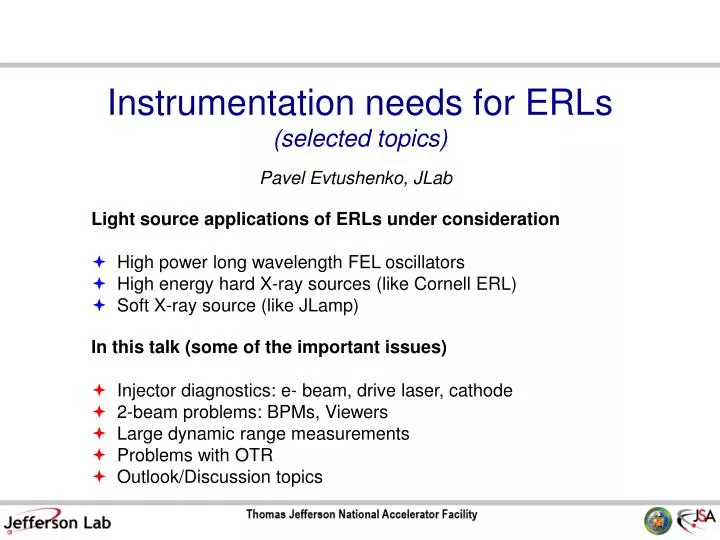
Instrumentation needs for ERLs (selected topics). Pavel Evtushenko, JLab. Light source applications of ERLs under consideration High power long wavelength FEL oscillators High energy hard X-ray sources (like Cornell ERL) Soft X-ray source (like JLamp).

E N D
Instrumentation needs for ERLs(selected topics) Pavel Evtushenko, JLab • Light source applications of ERLs under consideration • High power long wavelength FEL oscillators • High energy hard X-ray sources (like Cornell ERL) • Soft X-ray source (like JLamp) • In this talk (some of the important issues) • Injector diagnostics: e- beam, drive laser, cathode • 2-beam problems: BPMs, Viewers • Large dynamic range measurements • Problems with OTR • Outlook/Discussion topics
Gun / Injector diagnostics • There is a good overlap between the needs of different ERLs. • Such for any ERL we need to: • know the transverse phase space distribution • know the longitudinal phase space distribution • be able to measure and control halo • make sure that the beam parameters measured with pulsed beam do not • change when going to CW beams and changing the beam average current • know phase of the beam in RF cavities (1. setup 2. monitor) • have drive laser diagnostics • cathode (Q.E.) diagnostics
Injector / Transverse Phase Space The multislit or a single slit scanning through the beam (or a beam scanning across the slit) does the job very well (pulsed beam only). • well established technique • works for space charge dominated beam • beam profile is measured with YAG, phosphor or ceramic viewer • measures not only the emittance but the Twiss parameters as well • enough information to reconstruct the phase space • has been implemented as on-line diagnostics • works with diagnostics mode only (low duty cycle, average current)
Injector / Longitudinal Phase Space • Single cell cavity or multi-cell structure with TM dipole mode impose on the bunch • time dependent transverse kick. • The dipole creates dispersion in the transverse direction perpendicular to the • cavity kick • Problems: • the same as multislit – pulsed • beam only • resolution limited by transverse • emittance; solution – put a small • hole in front of the cavity and do • the measurements for small beamlet • AND as f(x,y) - 3D charge distribution • usually a special setup placed at the • beam line for injector study and • removed when it is done.
Injector / Drive Laser Diagnostics • Transversal profile of the D.L. on the cathode (standard technique) • imaging reflection from the input window to a CCD placed on the same • distance from the window as the cathode • Longitudinal profile: • auto-correlation works well for Gaussian pulses • for non Gaussian pulses streak camera (dynamic range ~103) • Amplitude stability: • photo diode (at JLab FEL is monitored all the time in control room) • Transversal stability: • long term slow drifts or misalignment – the same CCD as for profile meas. • fast transverse jitter 4-quadrant position sensitive photodiode • Phase stability (phase noise) all the way down to DC • fast (few GHz) photodiode to look at FM at very high harmonic number • BUT also must do measurements at DC to separate AM from FM • + Signal Source Analyzer (SSA) expansive but saves a lots of time
Injector / Drive Laser Diagnostics Typical auto-correlator signal JLab FEL D.L. (observed in the control room permanently) now the dynamic range can be few 1000 Courtesy of S. Zhang Drive Laser transverse profile dynamic range ~500: 10-bit frame grabber, 60 dB SNR CCD
Injector / Cathode Q.E. • For accurate modeling of the injector beam dynamics the input in to a code • must be accurate. This includes the emission transversal profile, which is a • product of the DL transverse distribution and QE transverse distribution • One technique to measure the Q.E. profile is scanner with a laser (spot on the • cathode is much smaller than cathode dimensions) and two scanning mirrors. • Usually automated and gives 2D distribution of the Q.E. Can be used only with • beam and gun voltage off. • Another technique: run low current emittance dominated beam, • measure the laser trans. profile and image the cathode to a view screen. • The ration of the beam profile and the laser profile gives Q.E. profile. • If used with the real drive laser (not always possible) gives the emission profile. QE scanner data Laser profile on cathode Photoemission profile
2-pass BPM (ideas) • Motivation: • To do differential orbit measurements • (measure transport matrix) with both • beams in the LINAC • The decelerating beam gets adiabatically • anti-dumped – small errors corrections in • the beginning leads to big orbit change at • the end • Orbit stabilization and feedback Stripline BPM signal measured with scope, the picture limited by the scope BW • V. Lebedev proposed at ERL05 to make a system based on small AM of the beam • current: switch the mod. frequency every turn, measure sidebands • Time domain approach might be very different for different machines • ✔ long recirculation time vs. short; ✔ every bucket filled vs. not • The phase difference is not always 180 deg, especially when tuning machine • In JLab FEL the ΔT between two beam depends on rep. rate.; smallest is 6 ns; • Time domain approach: (will not measure every bunch) • 1. make BPM pulses broader to 1.5 ns (LPF or dispersion) • 2. grab peak value with S&H (GHz BW) • 3. digitize S&H output with
2-pass viewers • there are two beams in the LINAC • when trying to measure decelerating • beam with a viewer the accelerating • beam gets also intercepted • ultimately the measurements should • be done with non intercepting technique • (or intercepting but negligibly ) • JLab FEL uses OTR viewers with 5 mm • hole (first beam goes in to the hole) • SRF cavities see the radiation due to • the intercepted beam (can trip cavity) JLab FEL LINAC OTR viewer • With the ultra bright beam OTR might be useless (OTR COTR like @ LCLS) • The best solution might be to use wire scanners (intercepts small part of the beam). • If the scanner measures radiation created by the wire, must take care of the background. • Laser wire scanner: • Will the measurements time and cost be acceptable? • What is the lowest energy when the technique is practical? • JLab FEL will test with beam: • 1. Electroformed mesh: 44% transparent ~5 micron thin • 2. Diamond-like carbon foils ~ 1 micron thin
Large dynamic range beam profile measurements Measured in JLab FEL injector, local intensity difference of the core and halo is about 300. (500 would measure as well) 10-bit frame grabber & a CCD with 57 dB dynamic range PARMELA simulations of the same setup with 3e5 particles: X and Y phase spaces, beam profile and its projection show the halo around the core of about 3e-3. Even in idealized system (simulation) beam dynamics can lead to formation of halo.
Large dynamic range measurements (example) • Main principal of one of the ways to make large dynamic range measurements is to reduce a measurement to frequency measurements. • Then make it work for 1 Hz and for 100 MHz and this is 108 dynamic range. • For instance use PMT and keep them working in counting mode. • Can be applied to e- beam measurements, laser, (light), X-rays. • Example: wire scanner measurements: Courtesy of A. Freyberger (measured at CEBAF)
LINAC beams are different from ring beams • JLab FEL transversal beam profile: • Obtained in a specially setup measurements to show how much beam is non Gaussian • It in not how we have it during standard operation • There is no Halo shown in this measurements in sense that all of it participates in FEL • interaction • The techniques we can borrow from rings assume Gaussian beam and therefore • are concentrating on beam size (RMS) measurements
Drive Laser large dynamic range measurements • typically in simulation the drive laser pulse is assumed “ideal” • i.e. as we want it • to find out how far is it true and if concerned about details of the phase • distribution at 1e-6 level, there is the need to make D.L. pulse • measurements with 1e6 dynamic range • transverse and longitudinal profile of the D.L. needs to be measured • measure and control reflections/scattering from D.L. transport; these might • be far from D.L. spot on the cathode both transversally and longitudinally • for transversal profile measurements: • could use 120 dB dynamic range CCD (2 CCD in one camera each 60 dB) • use a usual ~ 60 dB CCD with an ND filter and accurate cross-calibration • for longitudinal profile measurements: • auto-correlator with dynamic range 120 dB can be built using PMT • auto-correlator works fine for Gaussian pulses • WHAT to do for non Gaussian? Will cross-correlation work with 120 dB?
Drive Laser “ghost” pulses • For machine tune up, beam studies, intercepting diagnostics a “diagnostic • beam” with very low average current but nominal bunch charge is used • (all beam can be lost without damaging machine) • For example, JLab FEL: • max rep. rate 74.85 MHz (CW) • diagnostic mode: rep. rate 4.678125 MHz (÷16), 250 μs / 2 Hz (÷2000) • average current ~300 nA • Most of the laser pulses are “stopped” by EO cell(s), but the extinction ratio • of the an EO cell is about 200 (typical), two in series ~ 4×10⁴ • Another example: want to reduce 1300 MHz (100 mA) to 300 nA (218) • than for every bunch Qb we want • we also get 6.55×Qb of “ghost” pulses (655 % !!!) we do not want • “ghost” pulses overall intensity must be kept much lower than real pulses!!! • for “usual” measurements ~ 1% might be fine • much bigger problem if want to study halo, let’s say 10-6 effects, than • “ghost” pulses should be kept at 10-8 (???)
Drive Laser “ghost” pulses • Using a Log-amp is an easy way to diagnose presence of the “ghost” pulses • Log-amps with dynamic range 100 dB are available • Problem: • this does not work for CW beam current measurements with a linear circuit current measurements with A Log-amp circuit (60 dB)
Bright and small beams / COTR mitigation longitudinal BFF TR spectral power density of a bunch TR spectral power density of one electron transverse BFF BFF of a transversally Gaussian beam, when beam size σ>γλ/2π Q: How well will it work for planned ERLs? σ=200 micron Eb=250 MeV (LCLS) Courtesy of R. Fiorito (see PAC09 proceedings)
Fig. 1 Fig. 3 Fig. 4 Fig. 5
Pulsed and CW beam measurements / transition • Most affordable way to measure ps and • sub-ps bunches • Works with pulsed beam (tune up) and CW beam, essentially at any average current • Used at JLab FEL to ensure that the bunch length does not change for pulsed or CW and when the average current is increased • Ultimately needs to be setup in vacuum (or N2 purge) due to atmosphere absorption of THz • Phase information is lost – no direct bunch profile reconstruction • A detector measuring total CTR (CSR) power – a bunch length monitor interferogram Power spectrum
ERL Instrumentation Discussions • Diagnostics of high current CW beams especially at low energies in the injector region • is an area where we have least of experience: • - mostly beam profile measurements • - BPMs for beam position work • - bunch length (longitudinal profile) • At high energy outside of the LINAC can used SR the same way at the presently • operated high energy rings • - the BIG difference is that LINAC beams are not Gaussians, • since they are not in equilibrium • - pin hole cameras • - zone optics systems • - two slit interferometer with visible SR • Can not do that in the LINAC • - Can Optical Diffraction Radiation (ODR) be used (impedance) ? • - Laser wire (measurements time) ? • Make use of the fact that the beam is CW – very small modulation + lock-in amp
Conclusion and Outlook • For an injector transverse and longitudinal phase spaces can be measured • very well with pulsed (diagnostics) beams. • One direction to improve that is to increase the dynamic range of such • measurements to (106 – 108 ?) • In the injector area: how to deal with CW beam and transition from pulsed to • CW beam? What exactly will we need to deal with? • drifts in RF phase and amplitude – for sure!!! • beam loading ? Do we need beam based measurements for that? • wake fields? • measurements of D.L. with big dynamic range to understand beam dynamics • with the same big dynamic range • LINAC (part of the machine with 2 beams) needs specific solutions • reducing the CW beam to diagnostic beam needs careful consideration • this (via “ghost” pulses) affects all diagnostics
Conclusion and Outlook (2) • OTR (the working horse) will not be as easy to use as it used to be • need to mitigate COTR (experimental demonstration) • At the present light sources there is a lot of experience with SR diagnostics • for non distracting beam measurements. A lot of that can be applied to ERLs • with emittance ~ 10 times better. • Beam loss, fast shutdown systems • More topics for discussions • will the COTR mitigation work for ERL parameters? • for light sources: beam stability, orbit feedbacks – extend experience of 3rd • generation light sources and large scale LINACS • CW beam monitoring • Optical Diffraction Radiation (ODR) applicability • Transfer function (transverse and longitudinal) measurements and monitoring
The END (not really)
Again from SLAC-PUB-9280, courtesy of M. Ross “Foil” deformation – experiment OTR image of a beam ~ 10 m 10 m before (left) after (right) the OTR radiator was exposed to 51010 e-/train; rep. rate of the bunch trains 1.5 Hz for 5 minutes OTR radiator (initially) optically polished 500 m Be With ~ 10 time less charge per train for 30 min no degradation Suggested explanation – radiator deformation beyond elastic limit 51010e– 10077 pC bunches
unpolarized vertically polarized horizontally polarized Optical Diffraction Radiation amplitude of a Fourier component of transversal Coulomb field of an electron - transverse beam distribution intensity of the ODR from the beam Is 2D convolution of the fb and Er2 Example assuming 4.597 GeV; x=215 m; y=110 m; =550 nm; h=1.1 mm
It sounds simple, but it was debated till ~ 1996 • The reason for the debate was: transversal size of a Fourier component of a transversal component of Coulomb field of relativistic charged particle is: OTR resolution is diffraction limited K1 – modified Bessel function