Dynamic Causal Modelling (DCM)

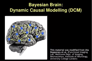
Dynamic Causal Modelling (DCM) Functional Imaging Lab Wellcome Dept. of Imaging Neuroscience Institute of Neurology University College London Presented by Uta Noppeney With Thanks to and Slides from Klaas Stephan Will Penny Karl Friston

System analyses in functional neuroimaging Functional specialisation Analyses of regionally specific effects: which areas constitute a neuronal system? Functional integration Analyses of inter-regional effects: what are the interactions between the elements of a given neuronal system? Functional connectivity = the temporal correlation between spatially remote neurophysiological events Effective connectivity = the influence that the elements of a neuronal system exert over another MODEL-free MODEL-dependent

Approaches to functional integration • Functional Connectivity • Eigenimage analysis and PCA • Nonlinear PCA • ICA • Effective Connectivity • Psychophysiological Interactions • MAR and State space Models • Structure Equation Models • Volterra Models • Dynamic Causal Models

Psychophysiological interactions Context X source target Set stimuli Context-sensitive connectivity Modulation of stimulus-specific responses source source target target

Approaches to functional integration • Functional Connectivity • Eigenimage analysis and PCA • Nonlinear PCA • ICA • Effective Connectivity • Psychophysiological Interactions • MAR and State space Models • Structure Equation Models • Volterra Models • Dynamic Causal Models

Overview • DCM – Conceptual overview • Neural and hemodynamic levels in DCM • Parameter estimation • Priors in DCM • Bayesian parameter estimation in non-linear systems • Interpretation of parameters • Bayesian model selection • Practical steps of a DCM study • Example: attention to visual motion

y y y y y The aim Functional integration and the modulation of specific pathways Contextual inputs Stimulus-free - u2(t) {e.g. cognitive set/time} BA39 Perturbing inputs Stimuli-bound u1(t) {e.g. visual words} STG V4 V1 BA37

Neuronal model Conceptual overview neuronal changes latent connectivity induced connectivity induced response Input u(t) The bilinear model c1 b23 neuronal states a12 activity z2(t) activity z3(t) activity z1(t) y y y Hemodynamic model BOLD

Conceptual overview • Models of • Responses in a single region • Neuronal interactions • Constraints on • Connections • Biophysical parameters Bayesian estimation posterior  likelihood ∙ prior

LG left FG right LG right FG left Example: linear dynamic system LG = lingual gyrus FG = fusiform gyrus Visual input in the - left (LVF) - right (RVF)visual field. z4 z3 z1 z2 RVF LVF u2 u1 systemstate input parameters state changes effective connectivity externalinputs

LG left FG right LG right FG left Extension: bilinear dynamic system z4 z3 z1 z2 CONTEXT RVF LVF u2 u3 u1

Bilinear state equation in DCM modulation of connectivity systemstate direct inputs state changes intrinsic connectivity m externalinputs

Neuronal model Conceptual overview neuronal changes latent connectivity induced connectivity induced response Input u(t) The bilinear model c1 b23 neuronal states a12 activity z2(t) activity z3(t) activity z1(t) y y y Hemodynamic model BOLD

The hemodynamic “Balloon” model • 5 hemodynamic parameters: important for model fitting, but of no interest for statistical inference • Empirically determinedprior distributions. • Computed separately for each area (like the neural parameters).

Overview • DCM – Conceptual overview • Neural and hemodynamic levels in DCM • Parameter estimation • Priors in DCM • Bayesian parameter estimation in non-linear systems • Interpretation of parameters • Bayesian model selection • Practical steps of a DCM study • Example 1: attention to visual motion

ηθ|y stimulus function u Overview:parameter estimation neural state equation • Combining the neural and hemodynamic states gives the complete forward model. • An observation model includes measurement errore and confounds X (e.g. drift). • Bayesian parameter estimationby means of a Levenberg-Marquardt gradient ascent, embedded into an EM algorithm. • Result:Gaussian a posteriori parameter distributions, characterised by mean ηθ|y and covariance Cθ|y. parameters hidden states state equation observation model modelled BOLD response

Overview:parameter estimation • Models of • Responses in a single region • Neuronal interactions • Constraints on • Connections • Biophysical parameters posterior  likelihood ∙ prior Bayesian estimation

needed for Bayesian estimation, embody constraints on parameter estimation express our prior knowledge or “belief” about parameters of the model hemodynamic parameters:empirical priors temporal scaling:principled prior coupling parameters:shrinkage priors Priors in DCM Bayes Theorem posterior  likelihood ∙ prior

Shrinkage priorsfor coupling parameters (η=0)→ conservative estimates! Priors in DCM • Principled priors: • System stability:in the absence of input, the neuronal states must return to a stable mode • Constraints on prior variance of intrinsic connections (A): Probability <0.001 of obtaining a non-negative Lyapunov exponent (largest real eigenvalue of the intrinsic coupling matrix) • Self-inhibition: Priors on the decay rate constant σ (ησ=1, Cσ=0.105); these allow for neural transients with a half life in the range of 300 ms to 2 seconds • Temporal scaling: Identical in all areas by factorising A and B with σ (a single rate constant for all regions): all connection strengths are relative to the self-connections.

Shrinkage Priors Small & variable effect Large & variable effect Small but clear effect Large & clear effect

Bayesian estimation: univariate Gaussian case Normal densities Univariate linear model Relative precision weighting

Bayesian estimation: multivariate Gaussian case General Linear Model Normal densities One step if Ce is known.

Current estimates Local linearization by 1st order Taylor: Likelihood Gradient ascent (Fisher scoring) with priors Friston (2002) NeuroImage, 16: 513-530. Bayesian estimation: nonlinear case Prior density

EM and gradient ascent • Bayesian parameter estimation by means of expectation maximisation (EM) • E-step:gradient ascent (Fisher scoring & Levenberg-Marquardt regularisation) to compute • (i) the conditional mean ηθ|y(= expansion point of gradient ascent), • (ii) the conditional covariance Cθ|y • M-step:Estimation of hyperparameters ifor error covariance components Qi: • Note: Gaussian assumptions about the posterior (Laplace approximation)

Parameter estimation: output in command window (new) E-Step: 1 F: -1.514001e+003 dp: 8.299907e-002 E-Step: 2 F: -1.200724e+003 dp: 9.638851e-001 E-Step: 3 F: -1.115951e+003 dp: 2.703493e-001 E-Step: 4 F: -1.077757e+003 dp: 2.002973e-002 E-Step: 5 F: -1.075699e+003 dp: 4.219233e-003 E-Step: 6 F: -1.075663e+003 dp: 1.030322e-003 E-Step: 7 F: -1.075661e+003 dp: 3.595806e-004 E-Step: 8 F: -1.075661e+003 dp: 2.273264e-006 Change of the norm of the parameter vector (= magnitude of update) objective function

ηθ|y Parameter estimation in DCM • Bayesian parameter estimation under Gaussian assumptions by means of EM and gradient ascent. • Result:Gaussian a posteriori parameter distributions with mean ηθ|y and covariance Cθ|y. • Combining the neural and hemodynamic states gives the complete forward model: • The observation model includes measurement error and confounds X (e.g. drift):

DCM parameters = rate constants Generic solution to the ODEs in DCM: Decay function: Half-life:

ηθ|y γ Interpretation of DCM parameters • Dynamic model (differential equations)  neural parameters correspond to rate constants (inverse of time constants  Hz!) speed at which effects take place • Identical temporal scaling in all areas by factorising A and B with σ:all connection strengths are relative to the self-connections. • Each parameter is characterised by the mean (ηθ|y) and covariance of itsa posteriori distribution. Its mean can be compared statistically against a chosen threshold γ.

ηθ|y γ Inference about DCM parameters:single-subject analysis • Bayesian parameter estimation in DCM: Gaussian assumptions about the a posteriori distributions of the parameters • Use of the cumulative normal distribution to test the probability by which a certain parameter (or contrast of parameters cT ηθ|y) is above a chosen threshold γ: • γ can be chosen as a function of the expected half life of the neural process, e.g. γ= ln 2 / τ

Inference about DCM parameters:group analysis • In analogy to “random effects” analyses in SPM, 2nd level analyses can be applied to DCM parameters: Separate fitting of identical models for each subject Selection of bilinear parameters of interest one-sample t-test:parameter > 0 ? paired t-test:parameter 1 > parameter 2 ? rmANOVA:e.g. in case of multiple sessions per subject

Pitt & Miyung (2002), TICS Model comparison and selection Given competing hypotheses on structure & functional mechanisms of a system, which model is the best? For which model i does p(y|mi) become maximal? Which model represents the best balance between model fit and model complexity?

Bayesian Model Selection Bayes theorem: Model evidence: Occam’s Razor: Ghahramani, Unsupervised Learning, 2004

Model evidence: Laplace approximation: The log model evidence can be represented as: Bayesian Model Selection

Bayesian information criterion (BIC): Akaike information criterion (AIC): Bayes factor: Approximations to model evidence Penny et al. 2004, NeuroImage

Hypothesis abouta neural system The DCM cycle Statistical test on parameters of optimal model Definition of DCMs as systemmodels Bayesian modelselection of optimal DCM Design a study thatallows to investigatethat system Parameter estimationfor all DCMs considered Data acquisition Extraction of time seriesfrom SPMs

Planning a DCM-compatible study • Suitable experimental design: • preferably multi-factorial (e.g. 2 x 2) • e.g. one factor that varies the driving (sensory) input • and one factor that varies the contextual input • Hypothesis and model: • define specific a priori hypothesis • Which alternative models? • which parameters are relevant to test this hypothesis? • TR: • as short as possible (optimal: < 2 s)

Timing problems at long TRs • Two potential timing problems in DCM: • wrong timing of inputs • temporal shift between regional time series because of multi-slice acquisition 2 slice acquisition 1 visualinput • DCM is robust against timing errors up to approx. ± 1 s • compensatory changes of σ and θh • Possible corrections: • restriction of the model to neighbouring regions • in both cases: adjust temporal reference bin in SPM defaults (defaults.stats.fmri.t0)

Practical steps of a DCM study - I • Conventional SPM analysis (subject-specific) • DCMs are fitted separately for each session → consider concatenation of sessions or adequate 2nd level analysis • Extraction of time series, e.g. via VOI tool in SPM • cave: anatomical & functional standardisation important for group analyses!

Practical steps of a DCM study - II • Possibly definition of a new design matrix, if the “normal” design matrix does not represent the inputs appropriately. • NB: DCM only reads timing information of each input from the design matrix, no parameter estimation necessary. • Definition of model • via DCM-GUI or directlyin MATLAB

Practical steps of a DCM study - III • DCM parameter estimation • cave: models with many regions & scans can crash MATLAB! • Model comparison and selection: • Which of all models considered is the optimal one? Bayesian model selection tool • Testing the hypothesisStatistical test onthe relevant parametersof the optimal model

Attention to motion in the visual system Stimuli 250 radially moving dots at 4.7 degrees/s Pre-Scanning 5 x 30s trials with 5 speed changes (reducing to 1%) Task - detect change in radial velocity Scanning(no speed changes) 6 normal subjects, 4 x 100 scan sessions; each session comprising 10 scans of 4 different conditions F A F N F A F N S ................. F - fixation point only A - motion stimuli with attention (detect changes) N - motion stimuli without attention S - no motion PPC V3A V5+ Attention – No attention Büchel & Friston 1997, Cereb. Cortex Büchel et al.1998, Brain

SPC V1 IFG V5 A simple DCM of the visual system Attention • Visual inputs drive V1, activity then spreads to hierarchically arranged visual areas. • Motion modulates the strength of the V1→V5 forward connection. • The intrinsic connection V1→V5 is insignificant in the absence of motion (a21=-0.05). • Attention increases the backward-connections IFG→SPC and SPC→V5. 0.55 0.26 0.72 0.37 0.56 0.42 Motion 0.66 0.88 -0.05 Photic 0.48 Re-analysis of data fromFriston et al., NeuroImage 2003

SPC SPC V1 V1 V5 V5 Comparison of three simple models Model 1:attentional modulationof V1→V5 Model 2:attentional modulationof SPC→V5 Model 3:attentional modulationof V1→V5 and SPC→V5 Attention Attention Photic Photic Photic SPC 0.55 0.03 0.85 0.86 0.85 0.70 0.75 0.70 0.84 1.36 1.42 1.36 0.89 0.85 V1 -0.02 -0.02 -0.02 0.56 0.57 0.57 V5 Motion Motion Motion 0.23 0.23 Attention Attention Bayesian model selection: Model 1 better than model 2, model 1 and model 3 equal → Decision for model 1: in this experiment, attention primarily modulates V1→V5

Neuronal model Summary neuronal changes latent connectivity induced connectivity induced response Input u(t) The bilinear model c1 b23 neuronal states a12 activity z2(t) activity z3(t) activity z1(t) y y y Hemodynamic model BOLD

Dynamic Causal Modelling (DCM)