Download
1 / 25
250 likes | 424 Views
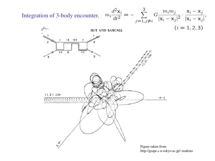
Integration of 3-body encounter. Figure taken from http://grape.c.u-tokyo.ac.jp/~makino. 4. Integration of Ordinary Differential Equations (ODE). We consider ODE with one variable, Most of results for this single ODE can be applicable for the above n-coupled ODE. A quick look for.

E N D
Integration of 3-body encounter. Figure taken from http://grape.c.u-tokyo.ac.jp/~makino
4. Integration of Ordinary Differential Equations (ODE). We consider ODE with one variable, Most of results for this single ODE can be applicable for the above n-coupled ODE.
A quick look for Existence, uniqueness, and stability of solution for ODE,
Exc 4-1) has a solution x(t) = t ( 1+ ln t). Apply Euler’s method changing the h = 1/2n , n=1 to 8, and estimate (a) the absolute error |yi - wi| at t = 6, and (b) the error ratio for the successive h = 1/2n at the same instant t = 6, namely, Exc 4-2) Perform the same analysis as 4-1) using the second order and fourth order Taylor methods. Because computations of higher derivatives is cumbersome, higher-order formula which involves evaluation f(t,y) only is more convenient.
Summary of the key concept on numerical method for ODE. • Local truncation error ti : The amount that the solution of ODE fails to • satisfy the the finite difference equation. • ex.) One-step method. • Global discretization error : • Definitions: (Consistency, Convergence and Stability)
One-step method. • One-step method is consistent if • Theorem: (Convergence and stability of the one-step method.) • Remark: Above theorem says • the one-step method is consistent ) convergent. It can be proved under the same conditions, the one-step method is convergent , consistent.
One-step method. • 2nd order Runge-Kutta method. • Determine constants a1, a2, d2, D2, so that f becomes O(h2) • approximation of the O(h2) Taylor method. • Modified Euler method. (Half step Euler + Midpoint integration.) • Heun method. (One step Euler + Trapezoidal integration.)
Optimal RK2 method. • Classical 4th order Runge-Kutta method. • Exc 4-3) Using an algebraic computing software, show that the local truncation error of Classical 4th-order Runge-Kutta method is O(h4).
Remarks on General s-stage Runge-Kutta method. • (1) For Explicit s-stage formula, it is not known in general what order O(hp) of formula one can construct for each level s. • (2) For Implicit s-stage formula, it is known that O(h2s) formula can be construct for each level s. • Formulas with properties (1) Small local truncation error, (2) Coefficients to be rational numbers, (3) many zeros in aj,l , are more practical. • Exc 4-4) Using the idea of Gauss-Legendre integration formula, derive 2-stage Runge-Kutta formula with 4th order accuracy.
Error control: Estimate the local truncation error and make it smaller than a certain threshold value by changing step size. • How to estimate the error ? • 1) Just to make h ! h/2. This is fine, but inefficient. • 2) Embedded formula. http://www.unige.ch/~hairer/software.html : for RK 8th order formula.
Linear (m-step) Multistep method. • Adams method: aj = 0, for j = 2, .. , m • Derivation: Integrating the both side of ODE, • Implicit linear multistep method is derived from interpolating polynomial of order m. • Explicit linear multistep method from interpolating polynomial of order m-1 • Substitute the form f(t,y(t)) = p(t) + R(t) in the integral form of ODE, and integrate it to calculate bj .
Explicit scheme is also called Adams-Bashforth, implicit Adams-Moulton. • Explicit scheme may be efficient since the f(ti,wi) of earlier steps are used. • The starting values for w0 (initial value), w1, …, wm-1 are required for the • m-step method. • These are calculated from one-step method of the same order. • For the implicit method, value at ti+1 , wi+1 , is calculated from an • algebraic equation. It is iteratively solved using wi+1 of an explicit • multistep method of the same order as an initial guess. • Usually this iteration is done by direct substitution, and only one or two • iteration is made. This procedure is called predictor – corrector schemes. • For this scheme, the 4th-order formula is the most popular.
In the Adams method, Newton form of polynomial interpolation formula is • used for changing the step size as well as the starting formula. • (Krogh type formula.) • The local truncation error estimation is often made by the difference • between predictor value and corrector value, which can be used for control • the step size h. • Exc4-5) Assuming uniform discretization in t domain, derive linear 2-step, 3-step 4-step explicit formulas and 1-step, 2-step, 3-step implicit formulas. Compare the coefficients of error terms between implicit and explicit formulas of the same order. • Exc4-6) Report on Krogh type formula. • Exc4-7) Report on the ODE solver that uses Richardson extrapolation.
Order of General Linear (m-step) Multistep method. • Conditions for the coefficients aj, and bJ to satisfy for having the local truncation error ti = O(hp) are written • Exc4-8) Derive these conditions. hint) Substitute dy/dt = f(t,y) to the equation for ti above, and expand y and y’ around t* = ti+1-m .
Consistency Convergence, and Stability of General Linear Multistep method. • Note: the starting values w1, …, wm-1 are assumed to be converge. • Consistency: (ti ! 0, as h ! 0) is satisfied if the local truncation error ti is a at least O(h).
Stability: Consider the case with f(t,y) = 0. • Definition: (Root condition) • The linear multistep method satisfies the Root condition if the zeros of the • associated characteristic polynomial • satisfy 1. • 2. • Theorem: (Stability) • A linear multistep method is stable if and only if it satisfies the root condition. • Definition: A stable multistep method is said to be strongly stable if l = 1 is the only zero of P(l) with | l | = 1, and to be weakly stable otherwise. • Remark: A linear multistep method that satisfies the consistency condition will always have at least one zero with l =1.
Convergence: 1. 2. 3. • Theorem: (Convergence) • A linear multistep method is convergent, if and only if it is both consistent and stable. .
Absolute stability and stiff equations. • Test problem: • This problem models a system of linear ODEs, in which case l represents an eigenvalue of the Jacobian associated with the r.h.s. • When the asymptotic character of a numerical approximation wn, n !1 matches that of exact solution y(t), t !1, the numerical method is said to be absolute stable. • One-step method:Consider the mth order Taylor methods. • Definition: The region of absolute stability for a one-step method is the set
Multistep method:Consider the linear m-step multistep method. • Definition: The region of absolute stability for a multistep method is the set • Exc 4-9) Derive the roots bk for 2-step Adams-Bashforth method and 2-step Adams Moulton method, and show the region of absolute stability on the complex plane.
Stiffness ratio: • Suppose {lk} is the set of characteristic expoennts associated with a particular ODE, stiffness ratio is defined by • Methods to efficiently compute a solution of stiff ODE are required to have • regions of absolute stability as large as possible. Possibly whole z < 0 plane. • Definition: (A-stable, Dahlquist) • A numerical method is A-stable if it is absolutely stable for all hl such that Re hl < 0. • Some known results: • Explicit Runge-Kutta methods are not A-stable. • Explicit linear multistep methods are not A-stable. • Order of A-stable implicit multistep methods is less than 2. • Among the A-stable implicit multistep methods, the trapezoidal method has the smallest local truncation error. • Any symmetric s-stage and O( h2s) order implicit Runge-Kutta method (implicit Gauss formula) are A-stable. Also Radau, Lobatto formulas.