Download
1 / 46
470 likes | 945 Views
Lossy Compression. CIS 658 Fall 2005. Lossy Compression. In order to achieve higher rates of compression, we give up complete reconstruction and consider lossy compression techniques So we need a way to measure how good the compression technique is

E N D
Lossy Compression CIS 658 Fall 2005
Lossy Compression • In order to achieve higher rates of compression, we give up complete reconstruction and consider lossy compression techniques • So we need a way to measure how good the compression technique is • How close to the original data the reconstructed data is
Distortion Measures • A distortion measure is a mathematical quality that specifies how close an approximation is to its original • Difficult to find a measure which corresponds to our perceptual distortion • The average pixel difference is given by the Mean Square Error (MSE)
Distortion Measures • The size of the error relative to the signal is given by the signal-to-noise ratio (SNR) • Another common measure is the peak-signal-to-noise ratio (PSNR)
Distortion Measures • Each of these last two measures is defined in decibel (dB) units • 1 dB is a tenth of a bel • If a signal has 10 times the power of the error, the SNR is 20 dB • The term “decibels” as applied to sounds in our environment usually is in comparison to a just-audible sound with frequency 1kHz
Rate-Distortion Theory • We trade off rate (number of bits per symbol) versus distortion this is represented by a rate-distortion function R(D)
Quantization • Quantization is the heart of any scheme • The sources we are compressing contains a large number of distinct output values (infinite for analog) • We compress the source output by reducing the distinct values to a smaller set via quantization • Each quantizer can be uniquely described by its partition of the input range (encoder side) and set of output values (decoder side)
Uniform Scalar Quantization • The inputs and output can be either scalar or vector • The quantizer can partition the domain of input values into either equally spaced or unequally spaced partitions • We now examine uniform scalar quantization
Uniform Scalar Quantization • The endpoints of partitions of equally spaced intervals in the input values of a uniform scalar quantizer are called decision boundaries • The output value for each interval is the midpoint of the interval • The length of each interval is called the step size • A UQT can be midrise or midtread
Uniform Scalar Quantization • Midtread quantizer • Has zero as one of its output values • Has an odd number of output values • Midrise quantizer • Has a partition interval that brackets zero • Has an even number of output values • For = 1
Uniform Scalar Quantization • We want to minimize the distortion for a given input source with a desired number of output values • Do this by adjusting the step size to match the input statistics • Let B = {b0, b1, …, bM } be the set of decision boundaries • Let Y = {y1, y2, …, yM } be the set of reconstruction or output values
Uniform Scalar Quantization • Assume the input is uniformly distributed in the interval [-Xmax, Xmax] • Then the rate of the quantizer is • R = log2M • R is the number of bits needed to code the M output values • The step size is given by = 2Xmax/M
Quantization Error • For bounded input, the quantization error is referred to as granular distortion • That distortion caused by replacing a whole range of values from a maximum values to ∞ (and also on the negative side) is called the overload distortion
Quantization Error • The decision boundaries bi for a midrise quantizer are • [(i - 1), i], i = 1 .. M/2 (for positive data X) • Output values yi are the midpoints • i - /2, i = 1.. M/2 (for positive data) • The total distortion (after normalizing) is twice the sum over the positive data
Quantization Error • Since the reconstruction values yiare the midpoints of each interval, the quantization error must lie within the range [-/2, /2] • As shown on a previous slide, the quantization error is uniformly distributed • Therefore the average squared error is the same as the variance (d)2 of from just the interval [0, ] with errors in the range shown above
Quantization Error • The error value at x is e(x) = x - /2, so the variance is given by (d)2 = (1/) 0 (e(x) - e)2dx (d)2 = (1/) 0 [x - (/2) - 0]2dx (d)2 = 2/12
Quantization Error • In the same way, we can derive the signal variance (x)2 as (2Xmax)2/12, so if the quantizer is n bits, M = 2nthen SQNR = 10log10[(x)2/(d)2] SQNR = 10log10 {[(2Xmax)2/12][12/2]} SQNR = 10log10 {[(2Xmax)2/12][12/ (2Xmax)2]} SQNR = 10log10M2 = 20n log102 SQNR = 6.02n dB
Nonuniform Scalar Quantization • A uniform quantizer may be inefficient for an input source which is not uniformly distributed • Use more decision levels where input is densely distributed • This lowers granular distortion • Use fewer where sparsely distributed • Total number of decision levels remains the same • This is nonuniform quantization
Nonuniform Scalar Quantization • Lloyd-Max quantization • iteratively estimates optimal boundaries based on current estimates of reconstruction levels then updates the level and continues until levels converge • In companded quantization • Input mapped using a compressor function G then quantized using a uniform quantizer • After transmission, quantized values mapped back using an expander function G-1
Companded Quantization • The most commonly used companders are u-law and A-law from telephony • More bits assigned where most sound occurs
Transform Coding • Reason for transform coding • Coding vectors is more efficient than coding scalars so we need to group blocks of consecutive samples from the source into vectors • If Y is the result of a linear transformation T of an input vector X such that the elements of Y are much less correlated than X, then Y can be coded more efficiently than X.
Transform Coding • With vectors of higher dimensions, if most of the information in the vectors is carried in the first few components we can roughly quantize the remaining elements • The more decorrelated the elements are, the more we can compress the less important elements without affecting the important ones.
Discrete Cosine Transform • The Discrete Cosine Transform (DCT) is a widely used transform coding technique • Spatial frequency indicates how many times pixel values change across an image block • The DCT formalizes this notion in terms of how much the image contents change in correspondence to the number of cycles of a cosine wave per block
Discrete Cosine Transform • The DCT decomposes the original signal into its DC and AC components • Following the techniques of Fourier Analysis, any signal can be described as a sum of multiple signals that are sine or cosine waveforms at various amplitudes and frequencies • The inverse DCT (IDCT) reconstructs the original signal
Definition of DCT • Given an input function f(i, j) over two input variables, the 2D DCT transforms it into a new function F(u, v), with u and v having the same range as i and j. The general definition is • Where i,u = 0, 1, … M-1, j, v = 0, 1, … N-1; and the constants C(u) and C(v) are defined by:
Definition of DCT • In JPEG, M = N = 8, so we have • The 2D IDCT is quite similar • with i,j, u, v = 0, 1, …,7
Definition of DCT • These DCTs work on 2D signals like images. • For one dimensional signals we have
Basis Functions • The DCT and IDCT use the same set of cosine functions - the basis functions
DCT Examples • The first example on the previous slide has a constant value of 100 • Remember - C(0) = sqrt(2)/2 • Remember - cos(0) = 1 • F1(0) = [sqrt(2)/(22)] (1100 +1100 + 1100 + 1100 + 1100 +1100 + 1100) 283
DCT Examples • For u = 1, notice that cos(/16) = -cos(15/16), cos(3/16)= -cos(13/16), etc. Also, C(1). So we have: • F1(1) = (1/2) [cos(/16) 100 + cos(3/16) 100 + cos(5/16) 100 + cos(7/16) 100 + cos(9/16) 100 + cos(11/16) 100 + cos(13/16) 100 + cos(15/16) 100] = 0 • The same holds for F1(2), F1(3), …, F1(7) each = 0
DCT Examples • The second example shows a discrete cosine signal f2(i) with the same frequency and phase as the second cosine basis function and amplitude 100 • When u = 0, all the cosine terms in the 1D DCT equal 1. • Each of the first four terms inside of the parentheses has an opposite (so they cancel). • E.g. cos /8 = -cos 7/8
DCT Examples • F2(0) = [sqrt(2)/(22)] 1 [100cos(/8) + 100cos(3/8) + 100cos(5/8) + 100cos(7/8) + 100cos(9/8) + 100cos(11/8) + 100cos(13/8) + 100cos(15/8)] • = 0 • Similarly, F2(1), F2(3), F2(4), …, F2(7) = 0 • For u = 2, because cos(3/8) = sin(/8) • we have cos2(/8) + cos2(3/8) = cos2(/8) + sin2(/8) = 1 • Similarly, cos2(5/8) + cos2(7/8) = cos2(9/8) + cos2(11/8) = cos2(13/8) + cos2(15/8) = 1
DCT Examples • F2(2) =1/2 [cos(/8) cos(/8) + cos(3/8) cos(3/8) + cos(5/8) cos(5/8) + cos(7/8) cos(7/8) + cos(9/8) cos(9/8) + cos(11/8) cos(11/8) + cos(13/8) cos(13/8) + cos(15/8) + cos(15/8)] 100 • = 1/2 (1 + 1 + 1 + 1) 100
DCT Characteristics • The DCT produces the frequency spectrum F(u) corresponding to the spatial signal f(i) • The 0th DCT coefficient F(0) is the DC coefficient of f(i) and the other 7 DCT coefficients represent the various changing (AC) components of f(i) • 0th component represents the average value of f(i)
DCT Characteristics • The DCT is a linear transform • A transform is linear iff • Where and are constants and p and q are any functions, variables or constants.
Cosine Basis Functions • For better decomposition, the basis functions should be orthognal, so as to have the least amount of redundancy • Functions Bp(i) and Bq(i) are orthognal if • Where “.” is the dot product
Cosine Basis Functions • Further, the functions Bp(i) and Bq(i) are orthonormal if they are orthognal and • Orthonormal property guarantees reconstructability • It can be shown that
2D Separable Basis • With block size 8, the 2D DCT can be separated into a sequence of 2 1D DCT steps (Fast DCT) • This algorithm is much more efficient (linear vs. quadratic)
Discrete Fourier Transform • The DCT is comparable to the more widely known (in mathematical circles) Discrete Fourier Transform
Other Transforms • The Karhunen-Loeve Transform (KLT) is a reversible linear transform that optimally decorrelates the input • The wavelet transform uses a set of basis functions called wavelets which can be implemented in a computationally efficient manner by means of multi-resolution analysis