Chapter 5: Valuation of Forwards & Futures

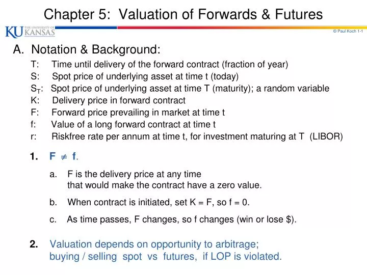
1. Chapter 5: Valuation of Forwards & Futures A. Notation & Background: T: Time until delivery of the forward contract (fraction of year) S: Spot price of underlying asset at time t (today) ST: Spot price of underlying asset at time T (maturity); a random variable K: Delivery price in forward contract F: Forward price prevailing in market at time t f: Value of a long forward contract at time t r: Riskfreerate per annum at time t, for investment maturing at T (LIBOR) 1.F  f. a. F is the delivery price at any time that would make the contract have a zero value. b. When contract is initiated, set K = F, so f = 0. c. As time passes, F changes, so f changes (win or lose $). 2. Valuation depends on opportunity to arbitrage; buying / selling spot vsfutures, if LOP is violated.

2. A. Notation & Background 3. Shorting the spot asset is different from shorting futures. Shorting futures is just like going long futures. Positions are symmetric. Each is simply a promise- to buy or sell - at a price agreed upon today, but deliver sometime in the future. Besides margin & marking-to-market, no cash is paid today. Shorting the spot – selling today something you don’t own. Today:must borrow asset from someone else, and then sell it. Receive proceeds of the sale now. This money is your asset; earns interest while you wait. Your liability is fact that you owe the asset & all its benefits (like dividends) to the original owner. Must maintain a margin account to protect against losses. Later: buy the asset back, and give it back to owner. If price ↓, make money. If price ↑, lose.

3. B. Forward Prices for a security that provides no income. e.g., discount bonds, non-dividend paying stocks, gold, silver 1. Example: T.Bill - sold at discount; pays $1,000,000 at mat. Suppose you wish to hold 151-day T. Bill. Two alternatives: Direct purchase: Buy 151-day T. Bill at S (today's spot price). Indirect purchase: Buy forward contract (at F) that delivers 91-day T. Bill in 60 days, and Buy 60-day T. Bill that will pay F in 60 days. |- - - - - - 91 days - - - - - -| Action day 0 60 days 151 days . Direct: Buy 151-day T. Bill S $1,000,000 Indirect: Buy forward contract -F $1,000,000 Buy 60-day T. Bill Fe -rT +F . . Sum of Cash FlowsFe -rT 0 $1,000,000 . Produce identical cash flows in 151 days; Should have same cost today. Pricing relation 1: Fe-rT = S ; orF* = SerT. Point : The forward offers something the spot purchase doesn’t, use of your money during life of forward; so erT pushes F higher.

4. B. Forward Prices for a security that provides no income. 2. Arbitrage Forces make pricing relation hold, if F is too high. a. Suppose F > S erT. i. F is too high relative to S; Buy at Sand sell at F. today ii. Borrow $Sand buy security. (Will owe $SerTat expiration.) Short a forward on the security. exp. iii. Exercise forward contract; deliver security for $F. Use part of proceeds to pay back loan, SerT; Keep diff., [F- SerT]. 3. Example: Forward contract on non-dividend paying stock; T = .25 (3 months); S = $40; r = .05 a. What should F be? F* = SerT= $40 e .05(.25) = $40.50 i. Suppose F = $43. F is too high relative to S ( F > S erT). today ii. Borrow $40 and buy the stock. (Will owe $40.50 at expiration.) Short a forward on the stock. exp. iii. Exercise forward contract; deliver stock for $43. Use part of proceeds to pay back loan, $40.50; Keep diff., $2.50

5. B. Forward Prices for a security that provides no income. 4.Arbitrage Forces make pricing relation hold, if F is too low. a. Suppose F < S erT. i. Fis too low relative to S; Sell at S and buy at F. today ii. Short the security, receive $S. Invest proceeds at r. (Will have SerT.) Buy a forward on the security. exp. iii. Proceeds worth $S erT.Use proceeds to exercise fwd (buy at $F). Deliver security to close out short sale; Keep diff., [SerT- F]. 5. Example: Forward contract on non-dividend paying stock; T = .25 (3 months); S = $40; r = .05 a. What should F be? F* = SerT= $40 e .05(.25) = $40.50 i. Suppose F = $39. F is too low relative to S ( F <S erT). today ii. Short the stock, receive $40. Invest proceeds at r. Buy a forward on the stock. exp. iii. Proceeds worth $40.50 ; Use proceeds to exercise fwd (buy at $39). Deliver stock to close out short sale; Keep diff., $1.50

6. C. Forward Prices on a security paying a known income. e.g., coupon-bearing bonds, dividend-paying stocks. 1. Example #1: T. Bond (pays coupons + face value at mat.). **Assume T. Bond pays no coupon during next 60 days. Two alternatives: Direct Purchase: Buy T. Bond at S (today's spot price). Indirect Purchase: Buy forward (at F) that delivers a T. Bond in 60 days, and Buy 60-day T. Bill that will pay F in 60 days. Action day 0 60 days future . Direct: Buy T. Bond Scoupons + face value Indirect: Buy forward contract -F coupons + face value Buy 60-day T. Bill Fe -rT +F .. Sum of Cash Flows Fe -rT 0 coupons + face value . Produce identical cash flows in future; Should have same cost today. Pricing relation 1: Fe-rT = S ; or F* = SerT. ** Same as B., since this T. Bond pays no income during life of forward.

7. C. Forward Prices on a security paying a known income. 2.Example #2: T. Bond (pays coupons + face value at mat.). **Now assume T. Bond pays coupon during next 60 days. Two alternatives: Direct Purchase: Borrow $I, and use this to help buy T. Bond. Must put up ($S - $I) today. Then coupon pays off loan. Indirect Purchase: Buy forward (at F) that delivers a T. Bond in 60 days, and Buy 60-day T. Bill that will pay F in 60 days. Action day 0 60 days future . Direct: Borrow $I and use coupon remaining coupons to help Buy T. Bond S - I pays loan plus face value Indirect: Buy forward contract -F remaining coupons Buy 60-day T. Bill Fe -rT +F . plus face value . Sum of Cash Flows Fe -rT0 remaining coupons + FV. Pricing relation 2: Fe -rT= S - I ; or F* = (S - I)erT. ** Point: Now two forces at work: 1. The forward offers something the spot purchase doesn’t, the use of your money during life of forward; so erT pushes F higher. 2. The spot purchase offers something the forward doesn’t, the first coupon; so $I pushes F lower.

8. D. Forward Prices on a security paying known dividend yield. 1. Let q = annual dividend yield, paid continuously. (e.g., stock indexes, foreign currencies.) Pricing Relation 3: F* = Se (r-q) T. If pricing relation does not hold, arbitrage opportunities: a. Buy e -qT (< 1) units of security today. b. Reinvest dividend income into more of security. c. Short a forward contract. This amount of the security grows at rate q; therefore, e -qTx eqT= 1 unit of security is held at expiration. Under forward contract, this security is sold at expiration for F. initial outflow = Se -qT; final inflow = F. Today, initial outflow = PV(final inflow). Thus, Se -qT= Fe -rT or F* = Se (r-q)T.

9. D. Forward Prices on a security paying known dividend yield. Pricing Relation 3: F* = Se(r-q) T. 2. Suppose F > Se (r-q) T. a. F is too high relative to S; Buy at S and sell at F. today b. Borrow $Se -qT and buy e -qT (< 1) units of the security. At expiration, will owe $Se -qTx erT= $Se (r-q) T. Short a forward on the security (promise to sell for F). then c. Security will provide dividend income at rate, q; Reinvest the dividend income into more of the security. exp. d. Now hold one unit of the security. Exercise forward contract; deliver security for $F. Use proceeds to pay off the loan. Keep diff., [ F - Se (r-q) T ].

10. D. Forward Prices on a security paying known dividend yield. Pricing Relation 3: F* = Se(r-q) T. 3. Similar formula to C. Two forces at work: a. The forward offers something the spot purchase doesn’t, use of your money during the life of the forward; so erT is pushing F higher. b. The spot purchase offers something the forward doesn’t, continuous stream of dividends at rate, q; so e -qt is pushing F lower.

11. E. General Formula for Valuation of Futures General Pricing Relation, true for all assets. The relation between f = (F - K)e -rTcurrent futures price (F) & delivery price (K), in terms of spot price (S) & K. 1. Explanations. a. Expl#1: If not, then arbitrage opportunities. b. Expl#2: When forward contract is entered, set F = K; f = 0. Later, as S changes, the appropriate value of F changes and f will become positive or negative. As F moves away from K, value (f) moves away from 0.

12. E. General Formula for Valuation of Futures 2. Consider formula in above cases: f = (F - K)e -rT a. security that provides no income. F* = SerT, so that f = (SerT- K)e –rT or f = S - Ke -rT. b. security that provides a known income. F* = (S-I)erT, so f = [(S-I)erT- K]e -rT or f = S - I - Ke -rT. c. security that pays a known dividend yield. F* = Se (r-q)T, so f = [Se (r-q)T- K]e -rTor f = Se -qT- Ke -rT. d. Note: in each case, the forward price at the current time (F) is the value of K that makes f = 0.

13. F. Applications – Stock Index Futures 1. Stock Index Futures. a. Examples of underlying asset - the stock index: i. S&P 500 - 400 industrials, 40 utilities, 20 transpco’s, and 40 banks. Companies amount to  80% of total mkt cap on NYSE. Two contracts traded on CME: i. $250 x index; ii. $50 x index. ii. S&P Midcap 400 - composed of middle-sized companies. Futures traded on CME. One contract is on $500 x index. iii. Nikkei 225 - largest stocks on TSE. Traded on CME. One contract is on $5 x index. iv. NYSE Composite Index - all stocks listed on NYSE. Traded on NYFE. One contract is on $250 x index. v. Nasdaq 100 - 100 Nasdaq stocks. Two contracts traded on CME: One is on $100 x index; Other (mini-Nasdaq) is on $20 x index. vi. International - CAC-40 (Euro stocks), DJ Euro Stoxx 50 (Euro stocks), DAX-30 (German stocks), FT-SE 100 (UK stocks).

14. F. Applications – Stock Index Futures b. Valuation. Consider S&P 500 futures. Treat as security with known dividend yield. Pricing Relation 3: F* = Se (r-q)T where q = average dividend yield. Problem 5.10. The risk-free rate of interest is 7% per annum with continuous compounding, and the avg dividend yield on a stock index is 3.2% p.a. The current value of the index is 150. What is the six-month futures price?Using the above equation, the six-month futures price is F* = 150 e(.07 - .032) x 0.5= $152.88.

15. G. Forward Prices on Foreign Currency Futures 1. Valuation -- 2 different explanations: a. Treat FC as security with known dividend yield, q = rf: (American terms – $/FC.) Pricing Relation 4:F* = Se (r - rf) T. Interest Rate Parity. b. Consider two alternative ways to hold riskless debt: i. U.S. riskless debt: $1  $1e r T - $ in one year ii. Foreign riskless debt [3 steps]: a) $1 / S - FC today b) ($1 / S) x erf T - FC in one year c) ($1 / S) x erf Tx F - $ in one year. Give same riskless cash flow in US$ in 1 year. So final $ outcome should be same. $1erT= [ ($1 / S) erf T ] F or erT= (F / S) erf T or F* = S e (r - rf) T. todayone year $:$1   1 erT$ _______________U.S. Riskless Debt_______________{ [ (1 / S) erf T ] F } $ || ( S)  ||(x F) | | FC:(1 / S) FC  Foreign Riskless Debt[ (1 / S) erf T ] FC

16. H. Commodity Futures Distinguish between commodities held solely for investment, and commodities held primarily for consumption. -- Arbitrage arguments used to value F for investment commodities, but only give upper bound for F for consumption commodities. 1.Gold and Silver (held primarily for investment). a. If storage costs = 0, like security paying no income: F* = S erT. b. If storage costs  0, costs can be considered as: i. Negative income. Let U = PV(storage costs); F* = (S + U) erT. ii. Negative div yield. Let u = % cost per annum; F* = S e(r + u) T. c. Point: Now two forces at work in same direction: i. Forward offers something spot purchase doesn’t, use of your money during life of forward; erTpushing F higher. ii. Forward offers something else spot doesn’t, no storage costs from holding spot; U pushing F higher.

17. H. Commodity Futures 2.Consumption commodities (not held for investmtpurposes). a. Suppose F > (S+U) erT.F too high. i. Borrow (S+U), buy 1 unit of commod. for S; pay storage costs; owe (S+U)erT at mat. ii. Short futures on 1 unit of commodity. Will give profit of [ F - (S+U)erT]. Can do this for any commodity. Arbitrage will force F down until equal (upper bound). b. Suppose F < (S+U)erT.F too low. i. Short 1 unit of comm., invest proceeds; save storage costs. Will have (S+U)erTat mat. ii. Buy futures on 1 unit of commodity. Will give profit of [ (S+U)erT - F ]. Can do this for gold and silver - held for investment. Arb. will force S down and F up. ** However, don't want to do this arbitrage for consumption commodities (if F too low). Commodity is kept in inventory because of its consumption value, not for investment. Cannot consume a futures contract! Thus, there are no arb. forces to eliminate inequality. For consumption commodities, F  (S+U) erT, or F  S e (r+u)T. Only have upper bounds for F on consumption commodities.

18. H. Commodity Futures For consumption commodity, F  (S+U)erT, or F  Se (r+u)T. 3.Convenience yield. a. Benefits from ownership of commodity not obtained with futures contract: (i) Ability to profit from temporary shortages. (ii) Ability to keep a production process going. b. If PV of storage costs (U) are known, Pricing Relation 7: then convenience yield, y, is defined so that: F eyT = (S+U) erT. c. If storage costs are constant prop. [u] of S, Pricing Relation 7: then convenience yield, y, is defined so that: F eyT = S e (r+u)T. d. Note: i. For consumption assets, ymeasures extent to which lhs < rhs. ii. For investment assets, y = 0, since arb. forces work both directions. iii. y reflects market's expectation avout future availability of commodity. If users have high inventories, shortages less likely & y should be smaller. If users have low inventories, shortages more likely, & yshould be larger. If y large enough, backwardation (F < S).

19. I. Cost of Carry 1. Definition: c = r + u - q = interest paid to finance asset + storage cost - income earned. a. For non-dividend paying stock, storage costs = income earned = 0; c = r; F* = Se r T; Cost of carry (c) = r. b. For stock index, storage costs = 0, & income earned at rate, q; c = r - q; F* = S e (r - q) T. This income ↓ c. c. For foreign currency, storage costs = 0, & income earned at rate, rf; c = r - rf; F* = Se (r - rf) T; This income ↓ c. d. For commodity, storage costs are like negative income at rate, u; c = r + u; F* = Se (r + u) T;These costs ↑ c. e.Summarizing: For investment asset, F = Se c T; (F > S by amount reflecting c.) For consumption asset, F = Se (c - y) T ; (F > S by amount reflecting the cost of carry, c, net of the convenience yield, y.)

20. J. Implied Delivery Options Complicate Things 1. Futures contracts specify delivery period. When during delivery period will the short want to deliver? a. Cost of Carry = c = (r + u - q) = (interest pd+ storage costs - income). b. Benefits from holding asset = (y + q - u) = (conv. yield + income - storage costs). c. If F is an increasing function of time, (F > S: contango), then r > (y + q - u). [Then F= Se (c - y) T; c - y > 0; c > y; (r - q + u) > y; r > y + q - u ]. Then it is usually optimal for short position to deliver early, since interest earned on cash (r) outweighs benefits of holding asset longer (y + q - u). ** Deliver early! Sell @ F (> S) ! Would rather have $F now! Start earning r now! d.If F is a decreasing function of time, (F < S: backwardation),then r < (y + q - u). [Then F= Se (c - y) T; c - y < 0; c < y; (r - q + u) < y; r < y + q - u ]. Then it is usually optimal for short position to deliver late, since benefits of holding asset longer (y + q - u) outweigh interest earned on cash (r). ** Deliver late! Sell @ F (< S) ! Would rather hold onto asset! Keep getting (y + q - u)!