Using the GFS Ensemble Mean to Generate Medium-range Precipitation Ensemble Forecasts for Hydrologic Ensemble Prediction

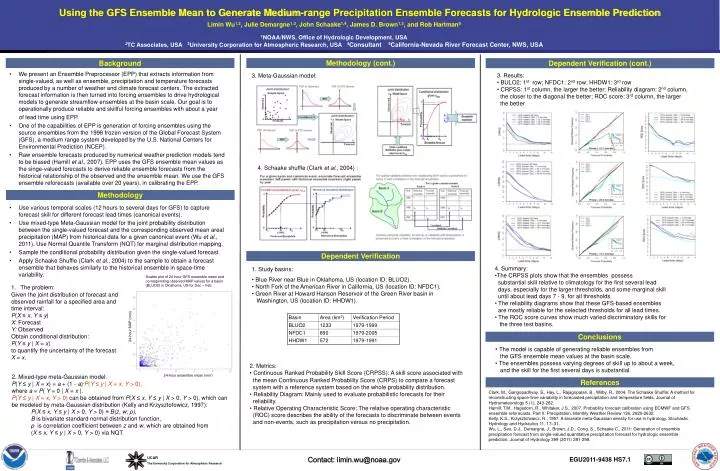
1. Using the GFS Ensemble Mean to Generate Medium-range Precipitation Ensemble Forecasts for Hydrologic Ensemble Prediction Limin Wu1,2, Julie Demargne1,3, John Schaake1,4, James D. Brown1,3, and Rob Hartman5 1NOAA/NWS, Office of Hydrologic Development, USA 2TC Associates, USA3University Corporation for Atmospheric Research, USA4Consultant 5California-Nevada River Forecast Center, NWS, USA Methodology (cont.) Background Dependent Verification (cont.) • We present an Ensemble Preprocessor (EPP) that extracts information from single-valued, as well as ensemble, precipitation and temperature forecasts produced by a number of weather and climate forecast centers. The extracted forecast information is then turned into forcing ensembles to drive hydrological models to generate streamflow ensembles at the basin scale. Our goal is to operationally produce reliable and skillful forcing ensembles with about a year of lead time using EPP. • One of the capabilities of EPP is generation of forcing ensembles using the source ensembles from the 1998 frozen version of the Global Forecast System (GFS), a medium range system developed by the U.S. National Centers for Environmental Prediction (NCEP). • Raw ensemble forecasts produced by numerical weather prediction models tend to be biased (Hamill et al., 2007). EPP uses the GFS ensemble mean values as the singe-valued forecasts to derive reliable ensemble forecasts from the historical relationship of the observed and the ensemble mean. We use the GFS ensemble reforecasts (available over 20 years), in calibrating the EPP. 3. Results: • BULO2: 1st row; NFDC1: 2nd row; HHDW1: 3rd row • CRPSS: 1st column, the larger the better; Reliability diagram: 2nd column, the closer to the diagonal the better; ROC score: 3rd column, the larger the better 3. Meta-Gaussian model: 4. Schaake shuffle (Clark et al., 2004) : Methodology • Use various temporal scales (12 hours to several days for GFS) to capture forecast skill for different forecast lead times (canonical events). • Use mixed-type Meta-Gaussian model for the joint probability distribution between the single-valued forecast and the corresponding observed mean areal precipitation (MAP) from historical data for a given canonical event (Wu et al., 2011). Use Normal Quantile Transform (NQT) for marginal distribution mapping. • Sample the conditional probability distribution given the single-valued forecast. • Apply Schaake Shuffle (Clark et al., 2004) to the sample to obtain a forecast ensemble that behaves similarly to the historical ensemble in space-time variability. Dependent Verification 4. Summary: • The CRPSS plots show that the ensembles possess substantial skill relative to climatology for the first several lead days, especially for the larger thresholds, and some marginal skill until about lead days 7 - 9, for all thresholds. • The reliability diagrams show that these GFS-based ensembles are mostly reliable for the selected thresholds for all lead times. • The ROC score curves show much varied discriminatory skills for the three test basins. 1. Study basins: • Blue River near Blue in Oklahoma, US (location ID: BLUO2). • North Fork of the American River in California, US (location ID: NFDC1). • Green River at Howard Hanson Reservoir of the Green River basin in Washington, US (location ID: HHDW1). Scatter plot of 24-hour GFS ensemble mean and corresponding observed MAP values for a basin (BLUO2) in Oklahoma, US for Dec – Feb. • The problem: Given the joint distribution of forecast and observed rainfall for a specified area and time interval: P(X ≤ x, Y ≤ y) X: Forecast Y: Observed Obtain conditional distribution: P(Y ≤ y | X = x) to quantify the uncertainty of the forecast X = x. 24-hour MAP (mm) Conclusions • The model is capable of generating reliable ensembles from the GFS ensemble mean values at the basin scale. • The ensembles possess varying degrees of skill up to about a week, and the skill for the first several days is substantial. 2. Metrics: • Continuous Ranked Probability Skill Score (CRPSS): A skill score associated with the mean Continuous Ranked Probability Score (CRPS) to compare a forecast system with a reference system based on the whole probability distribution. • Reliability Diagram:Mainly used to evaluate probabilistic forecasts for their reliability. • Relative Operating Characteristic Score: The relative operating characteristic (ROC) score describes the ability of the forecasts to discriminate between events and non-events, such as precipitation versus no precipitation. 2. Mixed-type meta-Gaussian model: P(Y ≤ y | X = x) = a + (1 - a)∙P(Y ≤ y | X = x, Y > 0), where a = P( Y = 0 | X = x ). P(Y ≤ y | X = x, Y > 0) can be obtained from P(X ≤ x, Y ≤ y | X > 0, Y > 0), which can be modeled by meta-Gaussian distribution (Kelly and Krzysztofowicz, 1997): P(X ≤ x, Y ≤ y | X > 0, Y > 0) ≈ B(z, w; ρ), B isbivariate standard normal distribution function, ρis correlation coefficient between z and w, which are obtained from (X ≤ x, Y ≤ y | X > 0, Y > 0) via NQT. 24-hour ensemble mean (mm) References Clark, M., Gangopadhyay, S., Hay, L., Rajagopalan, B., Wilby, R., 2004. The Schaake Shuffle: A method for reconstructing space-time variability in forecasted precipitation and temperature fields. Journal of Hydrometeorology 5 (1), 243-262. Hamill, T.M., Hagedorn, R., Whitaker, J.S., 2007. Probability forecast calibration using ECMWF and GFS ensemble reforecasts. Part II: Precipitation. Monthly Weather Review 136, 2620-2632. Kelly, K.S., Krzysztofowicz, R., 1997. A bivariate meta-Gaussian density for use in hydrology. Stochastic Hydrology and Hydraulics 11, 17–31. Wu, L., Seo, D.J., Demargne, J., Brown, J.D., Cong, S., Schaake C., 2011: Generation of ensemble precipitation forecast from single-valued quantitative precipitation forecast for hydrologic ensemble prediction. Journal of Hydrology 399 (2011) 281-298. EGU2011-9438 HS7.1 Contact: limin.wu@noaa.gov UCAR The University Corporation for Atmospheric Research