Correlation and Regression

1. Correlation and Regression

2. CORRELATIONS AND SCATTER PLOTS Scatter plots are used to show a relationship between 2 variables. Horizontal is the explanatory variable also called the control variable. Vertical is the response variable also know as the dependent variable.

3. Paired Data • is there a relationship? • if so, what is the equation? • use the equation for prediction

4. Looking at the scatter plot there should be some kind of pattern: • It should reveal: direction, form, and strength • Direction: the plotted points make a pattern that fall along positive or negative relationship. • Form: the points make some kind of oval shape to linear shape. • Strength: the closer the points are to a straight line determines the strength. • Outliers: outliers fall outside the pattern of the data, they deviate from the data.

5. Are there some concerns with this data?

6. Correlation measures the strength of the linear relationship between the two variables. • The goal is to see if there is a cause and affect between the two variables with a strong correlation coefficient. • If we find one then we will try to create a model for predicting values. Correlation exists between two variables when one of them is related to the other in some way

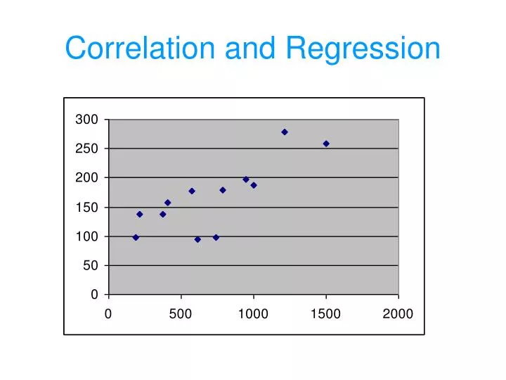
7. Does the appear to be a correlation between these two variables.

8. A noticeable Correlation does not mean a cause and affect.

9. Assumptions 1. The sample of paired data (x,y) is a random sample. 2. The pairs of (x,y) data have a bivariate normal distribution.

10. Definition • Scatterplot (or scatter diagram) is a graph in which the paired (x,y) sample data are plotted with a horizontal x axis and a vertical y axis. Each individual (x,y) pair is plotted as a single point.

11. Scatter Diagram of Paired Data

12. Positive Linear Correlation y y y x x x (a) Positive (b) Strong positive (c) Perfect positive Scatter Plots

13. Negative Linear Correlation y y y x x x (d) Negative (e) Strong negative (f) Perfect negative Scatter Plots

14. No Linear Correlation y y x x (h) Nonlinear Correlation (g) No Correlation Scatter Plots

15. Definition • Linear Correlation Coefficient r measures strength of the linear relationship between paired x and y values in a sample Calculators can compute r (rho) is the linear correlation coefficient for all paired data in the population.

16. Justification for r Formula Formula 9-1 is developed from  (x -x) (y -y) r= (x, y) centroid of sample points (n -1) Sx Sy x = 3 y x - x = 7- 3 = 4 (7, 23) • 24 20 y - y = 23 - 11 = 12 Quadrant 1 Quadrant 2 16 • 12 y = 11 (x, y) • 8 Quadrant 3 Quadrant 4 • • 4 FIGURE 9-6 x 0 0 1 2 3 4 5 6 7

17. Properties of the Linear Correlation Coefficient r 1. -1 r 1 2. Value of r does not change if all values of either variable are converted to a different scale. 3. The r is not affected by the choice of x and y. Interchange x and y and the value of r will not change. 4. r measures strength of a linear relationship.

18. Rounding the Linear Correlation Coefficient r • Round to three decimal places so that it can be compared to critical values in Table II (page A-2) • Use calculator or computer if possible

19. Critical Values of the Pearson Correlation Coefficient r = .01 n = .05 4 5 6 7 8 9 10 11 12 13 14 15 16 17 18 19 20 25 30 35 40 45 50 60 70 80 90 100 .950 .878 .811 .754 .707 .666 .632 .602 .576 .553 .532 .514 .497 .482 .468 .456 .444 .396 .361 .335 .312 .294 .279 .254 .236 .220 .207 .196 .999 .959 .917 .875 .834 .798 .765 .735 .708 .684 .661 .641 .623 .606 .590 .575 .561 .505 .463 .430 .402 .378 .361 .330 .305 .286 .269 .256 SEE PAGE A-2 IN APPENDIX

20. Interpreting the Linear Correlation Coefficient • If the absolute value of r exceeds the value in Table II, conclude that there is a significant linear correlation. • Otherwise, there is not sufficient evidence to support the conclusion of significant linear correlation.

21. = .01 n = .05 4 5 6 7 8 9 10 11 12 13 14 15 16 17 18 19 20 25 30 35 40 45 50 60 70 80 90 100 .950 .878 .811 .754 .707 .666 .632 .602 .576 .553 .532 .514 .497 .482 .468 .456 .444 .396 .361 .335 .312 .294 .279 .254 .236 .220 .207 .196 .999 .959 .917 .875 .834 .798 .765 .735 .708 .684 .661 .641 .623 .606 .590 .575 .561 .505 .463 .430 .402 .378 .361 .330 .305 .286 .269 .256 Does the appear to be a correlation between these two variables. r = .446

22. = .01 n = .05 4 5 6 7 8 9 10 11 12 13 14 15 16 17 18 19 20 25 30 35 40 45 50 60 70 80 90 100 .950 .878 .811 .754 .707 .666 .632 .602 .576 .553 .532 .514 .497 .482 .468 .456 .444 .396 .361 .335 .312 .294 .279 .254 .236 .220 .207 .196 .999 .959 .917 .875 .834 .798 .765 .735 .708 .684 .661 .641 .623 .606 .590 .575 .561 .505 .463 .430 .402 .378 .361 .330 .305 .286 .269 .256 A noticeable Correlation does not mean a cause and affect. r = .541

23. 250 200 150 100 50 0 1 2 3 4 5 6 7 8 0 Common Errors Involving Correlation FIGURE 9-2 Distance (feet) Time (seconds) Scatterplot of Distance above Ground and Time for Object Thrown Upward

24. Data from the Garbage Project x Plastic (lb) 0.27 2 1.41 3 2.19 3 2.83 6 2.19 4 1.81 2 0.85 1 3.05 5 y Household Is there a significant linear correlation?

25. Data from the Garbage Project x Plastic (lb) 0.27 2 1.41 3 2.19 3 2.83 6 2.19 4 1.81 2 0.85 1 3.05 5 y Household Is there a significant linear correlation? n = 8 Correlation Coefficient r = 0.842

26. = .01 = .05 n 4 5 6 7 8 9 10 11 12 13 14 15 16 17 18 19 20 25 30 35 40 45 50 60 70 80 90 100 .950 .878 .811 .754 .707 .666 .632 .602 .576 .553 .532 .514 .497 .482 .468 .456 .444 .396 .361 .335 .312 .294 .279 .254 .236 .220 .207 .196 .999 .959 .917 .875 .834 .798 .765 .735 .708 .684 .661 .641 .623 .606 .590 .575 .561 .505 .463 .430 .402 .378 .361 .330 .305 .286 .269 .256 Is there a significant linear correlation? n = 8 Correlation Coefficient r = 0.842 Critical values are r = - 0.707 and 0.707 (Table II with n = 8 and = 0.05) Since 0.842 is > 0.707 then this is a significant correlation. SEE PAGE A-2 IN APPENDIX IN SULLIVAN BOOK TABLE II Critical Values of the Pearson Correlation Coefficient r

27. END