Download
1 / 36
390 likes | 971 Views
Modeling and Analysis of Signal Estimation for Stepper Motor Control. Dan Simon Cleveland State University October 8, 2003. Outline. Problem statement Simplorer and Matlab Optimal signal estimation Postprocessing Simulation results Conclusion. Problem statement.

E N D
Modeling and Analysis of Signal Estimation forStepper Motor Control Dan SimonCleveland State UniversityOctober 8, 2003
Outline • Problem statement • Simplorer and Matlab • Optimal signal estimation • Postprocessing • Simulation results • Conclusion
Problem statement • Speed control for PM DC motor • Aerospace applications • Flywheel energy storage • Flight control trim surfaces • Hydraulics • Fans • Thrust vector control • Fuel pumps
Problem statement DC Machine Permanent Excitation I = armature current V = armature voltage L = inductance R = resistance k = motor constant • = rotor speed • = rotor angle J = moment of inertia TL = load torque
Problem statement State assignment: • x1 = I • x2 = • x3 = • x4 = TL / J Measurements: • y = current (and possibly position)
Problem statement Estimate velocity x2
Simplorer and Matlab • Simplorer • Circuit element models • Electric machine models • Data analysis tools • Interfaces with Matlab / Simulink
Simplorer and Matlab • Matlab • Powerful math and matrix capabilities • Co-Simulation • Link Simplorer and Matlab • Plot and analyze data in either environment
Simplorer and Matlab • Use the SiM2SiM tool inAdd Ons / interfaces6 • Begin the simulation in Simulink
Simplorer and Matlab Define Simplorer inputs and outputs in the property dialog of the SiM2SiM component Simplorer ↔ Simulink
Simplorer and Matlab • Use the S-function property dialog in Matlab to link Simplorer / Matlab signals
Simplorer and Matlab • Begin the simulation in Matlab • Couple Simplorer’s and Matlab’s strengths • Simplorer: power electronics, electromechanics, data analysis, state diagrams • Matlab: matrix algebra, toolboxes • Data analysis / viewing can be done in either Simplorer or Matlab
Optimal signal estimation Given a linear system: x = state y = measurement u = control input w, v = noise Find the best estimate for the state x
Optimal signal estimation Suppose w ~ N(0, Q) and v ~ N(0, R). The Kalman filter solves the problem
Optimal signal estimation The H filter solves the problem This is a game theory approach. Nature tries to maximize the estimation error. The engineer tries to minimize the error.
Optimal signal estimation Rewrite the previous equation: Game theory: nature tries to maximize J and the engineer tries to minimize J
Optimal signal estimation The H filter is given as follows: Note this is identical to the Kalman filter except for an extra term in the Riccati equation.
Optimal signal estimation • The Kalman filter is a least-mean-squares estimator • The H filter is a worst-case estimator • The Kalman filter is often made more robust by artificially increasing P • The H filter shows exactly how to increase P in order to add robustness
Optimal signal estimation • Steady state: Jacopo Riccati 1676-1754 • This is an Algebraic Riccati Equation • Real time computational savings
Transfer Matlab data to Simplorer for plotting and analysis Postprocessing
Postprocessing • Start the Matlab postprocessor interface before starting the co-simulation • After running the co-simulation, the Day postprocessor can exchange data with Matlab
Postprocessing Drag data between Day and Matlab Matlab variables Matlab output Matlab commands
Postprocessing • Day cannot handle arrays with more than two dimensions – use Matlab’s “squeeze” command • Make sure Matlab data is not longer than Simplorer’s time array
Simplorer data Postprocessing Matlab data
Postprocessing Analysis Characteristicsto view statistical information Select the desired output variable Export to table
Simulation results motor parameters control input measurements Ouput from Matlab
Simulation results motor PI Controller
Simulation results Simulation parameters: • 1.2 ohms, 9.5 mH, 0.544 Vs, 0.004 kgm2 • Initial speed = 0cmd speed = 1000 RPM • External load torque changes from 0 to 0.1 • Measurement errors 0.1 A, 0.1 rad (1 )
Simulation results Steady state parameters: • Initial speed = 1000commanded speed = 1000 RPM • External load torque = 0 • Measurement error = 0.1 A, 0.1 rad (1 )
Simulation results RMS Estimation Errors (RPM)current and position measurements
Simulation results Now suppose we measure winding current but not rotor position. Can we still get a good estimate of motor velocity?
Simulation results RMS Estimation Errors (RPM)current measurement only
Conclusion • Motor state estimation is required for motor control • Kalman filtering and H filtering can be used for motor state estimation • Steady state filtering saves time • Simplorer / Matlab co-simulation • Estimate motor parameters R, L, J, k