Download
1 / 33
330 likes | 541 Views
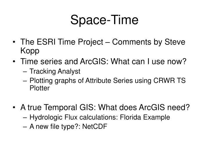
Space-Time. The ESRI Time Project – Comments by Steve Kopp Time series and ArcGIS: What can I use now? Tracking Analyst Plotting graphs of Attribute Series using CRWR TS Plotter A true Temporal GIS: What does ArcGIS need? Hydrologic Flux calculations: Florida Example

E N D
Space-Time • The ESRI Time Project – Comments by Steve Kopp • Time series and ArcGIS: What can I use now? • Tracking Analyst • Plotting graphs of Attribute Series using CRWR TS Plotter • A true Temporal GIS: What does ArcGIS need? • Hydrologic Flux calculations: Florida Example • A new file type?: NetCDF
Tracking Analyst • Simple Events • 1 feature class that describes What, When, Where • Complex Event • 1 feature class and 1 table that describe What, When, Where Arc Hydro
Simple Event Unique Identifier for objects being tracked through time Observation Time of observation (in order) Geometry of observation
Complex Event (stationary version) Cases 1, 2, 3, 4, 5 The object maintains its geometry (i.e. it is stationary)
Complex Event (dynamic version) Cases 6 and 7 The object’s geometry can vary with time (i.e. it is dynamic)
Tracking Analyst Demo • Show the Galveston Bay Monitoring Point feature class and Time Series Table • Show the temporal layer • Show the tracking analyst time “Playback Manager” • Animate bacteria concentrations
Variable Time Time and Space in GIS Time Series Feature Series t3 t2 Value t1 Time Attribute Series Raster Series Value t3 t2 t1 t1 t2 t3 y x
Variable Time t1 t2 t3 Time Series and Temporal Geoprocessing DHI Time Series Manager Time Series Feature Series t3 t2 Value t1 Time Attribute Series Raster Series Value t3 t2 t1 y x ArcGIS Temporal Geoprocessing Adobe picture
Arc Hydro Attribute Series TSDateTime Feature Class (point, line, area) TSValue FeatureID TSType TSType Table
Arc Hydro Attribute Series Feature Class (HydroID) Attribute Series Table (FeatureID)
Attribute Series Typing TSType Attribute Series • Map time series e.g. Nexrad • Collections of values recorded at various locations and times e.g. water quality samples • This is current Arc Hydro time series structure 1 * Type Units Regular …. Type Time FeatureID Value
Plotting Attribute Series • One feature with a time-dependent Attribute • Observed or Modeled • Complications • Regular or Irregular in time • Many Types (rainfall, streamflow, dissolved oxygen, etc.) • Instantaneous, cumulative, averaged, min, max, etc. • Different units (cfs, m3/d, gpd, etc.) • Plot the data in ArcMap
TS Plotter Demo • Show TSType Table • Plot time series for a few MonitoringPoint features • Summarize data into yearly averages • Export data and chart to Excel • Show exported data and chart in Excel
South Florida Water Management Project • Prototype region includes 24 water management basins, • More than 70 water control structures managed by the South Florida Water Management District (SFWMD) • Includes natural and managed waterways Prototype Area Lake Kissimmee Lake Istokpoga Lake Okeechobee
Questions that SFWMD wants Answered • How much water is there? • Where is the water in the District? • How much water will enter the canal system? • How can water be routed from one basin to another?
DBHydro TimeSeries Achieve of Water Related Time Series Data currently used by SFWMD Example of Flow Data: Daily Average Flow [cfs] at Structure S65 (spillway) Spatial Information About point of measurement Unique 5-digit alphanumeric code calledDBKEY Date/Time Value • DBHydro can be accessed at:http://www.sfwmd.gov/org/ema/dbhydro/index.html
Coupling Table: Linking Control Volume to Features Water Balance performed over a Control Volume (i.e.: Basin) Coupling Table links the Control Volume (basin) to all features that transfer water into and out of the Control Volume Horizontal (structures) Vertical (rainfall, ETp) Qin Qrain Qevap Qout S65BC Basin
Water Balancing in ArcHydro QS65A +QRAIN - QETp –QS65C = Storage
Coupling Table Design HydroID of Inflow or Outflow Feature that contains Time Series Information If Inflow/Outflow is a flux, include an area over which the flux acts HydroID of Control Volume Direction of Flow 1 = IN, 2 = OUT ObjectID
Demo of Flow and Flux Calculations using TSViewer Links Control Volume Feature with Inflow and Outflows
Multidimensional Data Representation for the Geosciences Atmospheric Science Hydrology Ocean Science Earth Science
Weather Information Continuous in space and time Combines data and simulation models Delivered in real time Hydrologic Information Static spatial info, time series at points Data and models are not connected Mostly historical data Weather and Hydrology • Challenges for Hydrologic Information Systems • How to better connect space and time? • How to connect space, time and models? • How to connect weather and hydrology?
Arc Hydro Attribute Series TSDateTime Feature Class (point, line, area) TSValue FeatureID TSType TSType Table
NetCDF Data Model (developed at Unidata for distributing weather data) Time Dimensions and Coordinates Value Space (x,y,z) NetCDF describes a collection of variables stored in a dimension space that may represent coordinate points in the (x,y,z,t) dimensions Variables Attributes
NetCDF File for Weather Model Output of Relative Humidity (Rh) dimensions: lat = 5, long = 10, time = unlimited; variables: lat:units = “degrees_north”; long:units = “degrees_east”; time:units = “hours since 1996-1-1”; data: lat = 20, 30, 40, 50, 60; long = -160, -140, -118, -96, -84, -52, -45, -35, -25, -15; time = 12; rh = .5,.2,.4,.2,.3,.2,.4,.5,.6,.7, .1,.3,.1,.1,.1.,.1,.5,.7,.8,.8, .1,.2,.2,.2,.2,.5,.7,.8,.9,.9, .1,.2,.3,.3,.3,.3,.7,.8,.9,.9 .0,.1,.2,.4,.4,.4,.4,.7,.8,.9; rh (time, lat, lon);
Interpolate to Raster GeoTiff format, cell size = 0.5º
Average Rh in each State Determined using Spatial Analyst function Zonal Statistics with Rh as underlying raster and States as zones
Integrated Data Viewer(Developed by Unidata) • Data Probe • Vertical Profile • Time/Height display • Vertical cross-section • Plan view • Isosurface Note: IDV = Integrated Data Viewer
RUC20 – Output Samples Precipitable water in the atmosphere Cross-section of relative humidity Wind vectors and wind speed (shading) Images created from Unidata’s Integrated Data Viewer (IDV)
IDV Demo For RUC20 predicted temperature (4D dataset) show: • Plan view changes over time • Cross-section changes over time • Vertical Profile changes over time • Data Probe changes over time