Download

1 / 33
330 likes | 336 Views
Image Compression. 1. Our eyes and ears cannot distinguish subtle change in signal’s parameter. In such cases, we can use a lossy data compression method.

E N D
Image Compression www.assignmentpoint.com 1
Our eyes and ears cannot distinguish subtle change in signal’s parameter. In such cases, we can use a lossy data compression method. JPEG (Joint Photographic Experts Group) encoding is used to compress pictures and graphics, MPEG (Moving Picture Experts Group) encoding is used to compress video, and MP3 (MPEG audio layer 3)for audio compression. www.assignmentpoint.com
Introduction • The goal of image compression is to reduce the amount of data required to represent a digital image. • i.e., remove redundant data from the image • Image compression is very important for image storage and image transmission. www.assignmentpoint.com
Approaches • Lossless • Information preserving • Low compression ratios • Lossy • Does not preserve information • High compression ratios • Tradeoff: image quality vs compression ratio www.assignmentpoint.com
Step-1 Formation of 8×8 blocks of Y, I and Q matrix Step-1 Step-1 of encoding an image with JPEG is block preparation. Let us assume that JPEG input is a 640×480 RGB image with 24 bis/pixel. Since using luminance and chrominance gives better compression, we first compute the luminance, Y and two chrominance I and Q (NTSC) using following formula. Y = 0.3R+0.59G+0.11B I = 0.6R-0.28G-0.32B Q = 0.21R-0.52G+0.31B www.assignmentpoint.com
Y, I and Q matrices R, G and B matrices Separate matrices are constructed for Y, I and Q each with elements in the range 0-255. Next, square blocks of four pixels are averaged in the I and Q matrices to reduce them to 320×240. This reduction is lossy, but the eye barely notices it since eye responds to luminance's more than chrominance www.assignmentpoint.com
RGB 640×480 Each pixel is of 24 bits y 640×480 Each pixel is of 8 bits I 320×240 Each pixel is of 8 bits Q 320×240 Each pixel is of 8 bits www.assignmentpoint.com
Finally each matrix is divided into 8×8 blocks www.assignmentpoint.com
The Y matrix has 4800 blocks and the other two have 1200 blocks y 640×480 Each pixel is of 8 bits I 320×240 Each pixel is of 8 bits Q 320×240 Each pixel is of 8 bits www.assignmentpoint.com
Now 128 is subtracted from each element of all three matrices t0 put 0 in the middle range. Subtracting -128 www.assignmentpoint.com
Step-2 Discrete Cosine Transform Step-2 of JPEG is to apply DCT to each of the 7200 blocks separately. The output of each DCT is 8×8 matrix of DCT coefficients. DCT element F(0,0) is the average value of the block called DC component. The other elements tell how much spectral power is presented at each spatial frequency www.assignmentpoint.com
Inverse DCT (IDCT) 88 two-dimensional separable IDCT: IDCT can be computed using the same routine as DCT www.assignmentpoint.com
8x8 DCT DC coefficient AC coefficients DCT 8x8 image block DCT coefficients Low frequencies Medium frequencies Increasing frequency High frequencies www.assignmentpoint.com
8x8 DCT 52 55 61 66 70 61 64 73 63 59 66 90 109 85 69 72 62 59 68 113 144 104 66 73 63 58 71 122 154 106 70 69 Pixel domain 67 61 68 104 126 88 68 70 79 65 60 70 77 68 58 75 85 71 64 59 55 61 65 83 87 79 69 68 65 76 78 94 DCT IDCT DC 609 - 29 - 62 25 55 - 20 - 1 3 7 - 21 - 62 9 11 - 7 - 6 6 - 46 8 77 - 25 - 30 10 7 - 5 Frequency domain - 50 13 35 - 15 - 9 6 0 3 AC 11 - 8 - 13 - 2 - 1 1 - 4 1 - 10 1 3 - 3 - 1 0 2 - 1 - 4 - 1 2 - 1 2 - 3 1 - 2 - 1 - 1 - 1 - 2 - 1 - 1 0 - 1 www.assignmentpoint.com
8X8 block of pixel values taken from original image Subtracting -128 DCT www.assignmentpoint.com
Step-3 Quantization Each co-efficient of 8×8 DCT matrix is divided by a weight taken from a table quantization (16 is the value of the first pixel from quantization matrix) www.assignmentpoint.com
8X8 block of pixel values taken from original image Subtracting -128 DCT quantization using −415 (the DC coefficient) and rounding to the nearest integer (16 is the value of the first pixel from quantization matrix) www.assignmentpoint.com
Quantization of DCT Coefficients Typical quantization matrices (may be altered depending on data) Original term Quantized term = round( ) Quantization factor Restored term = Quantized term * Quantization factor www.assignmentpoint.com
Step-4 DPCM and zigzag scanning Since DC values of each 8×8 matrix is the average value of the respective blocks therefore they change slowly. To obtain the small value we simply subtract the DC coefficient of the previously processed 8x8 pixel block from the DC coefficient of the current block. This value is called the "DPCM difference". No difference is computed from AC components. www.assignmentpoint.com
Now zig-zag scanning is done on each 8×8 matrix and run-length encoding is applied which generates a list of numbers. Finally Huff-encodes the numbers for storage or transmission. www.assignmentpoint.com
Zig-zag scan −26 −3 0 −3 −2 −6 2 −4 1 −4 1 1 5 1 2 −1 1 −1 2 0 0 0 0 0 −1 −1 0 0 0 0 0 0 0 0 0 0 0 0 0 0 0 0 0 0 0 0 0 0 0 0 0 0 0 0 0 0 0 0 0 0 0 0 0 0 www.assignmentpoint.com
JPEG compression www.assignmentpoint.com
Original Image JPEG 27:1 www.assignmentpoint.com
JPEG Compression Example • Original image • 512 x 512 x 8 bits = 2,097,152 bits • JPEG • 27:1 reduction =77,673 bits www.assignmentpoint.com
Transformation of image In this section first an RGB image will be read and it will be converted to an 8-bit grayscale and binary image. Finally both the images will be shown. %MATLAB code rgb = imread('onion.png'); %read the image subplot(2,2,1) imshow(rgb) title('(a)') I = rgb2gray(rgb);%convert the RGB to gray scale image subplot(2,2,2) imshow(I) title('(b)') BW = dither(I); subplot(2,2,3) imshow(BW) title('(c)') The results of the code are shown in fig.1. www.assignmentpoint.com
A = im2double(imread('rice.png')); subplot(2,1,1) imshow(A); title('Original Image') D = dctmtx(size(A,1)); dct = D*A*D'; subplot(2,1,2) imshow(dct) title('Image spectrum after DCT') DCT of an image www.assignmentpoint.com
I = im2double(imread('rice.png')); fun = @dct2; J = blkproc(I,[8 8],fun); imshow(J) DCT is applied on 8X8 block B = blkproc(A,[m n], fun) processes the image A by applying the function fun to each distinct m-by-n block of A, padding A with 0's if necessary www.assignmentpoint.com
Huffman Coding: Let us consider four symbols 1, 2, 3 and 4; a random sequence of symbols is [1 3 1 3 4 3 3 4 2 3 2 1] and their probability of occurrence, P=[3/12 2/12 5/12 2/12]. The symbol dictionary is created by the function huffmandict which is used to encode and decode using the huffmanenco and huffmandeco functions. sig = repmat([1 3 1 3 4 3 3 4 2 3 2 1],1,5); % random sequence of symbols and will be repeated 5 timessymbols = [1 2 3 4]; % set of symbolsp = [3/12 2/12 5/12 2/12]; % Probability of each symboldict = huffmandict(symbols,p); % Create the dictionary.hcode = huffmanenco(sig,dict); % Encode the data.dhsig = huffmandeco(hcode,dict); % Decode the code. www.assignmentpoint.com
DCT and Image Compression In the JPEG image compression algorithm, the input image is divided into 8-by-8 or 16-by-16 blocks, and the two-dimensional DCT is computed for each block. The DCT coefficients are then quantized, coded, and transmitted. The JPEG receiver (or JPEG file reader) decodes the quantized DCT coefficients, computes the inverse two-dimensional DCT of each block, and then puts the blocks back together into a single image. For typical images, many of the DCT coefficients have values close to zero; these coefficients can be discarded without seriously affecting the quality of the reconstructed image. www.assignmentpoint.com
I = imread('cameraman.tif'); I = im2double(I); T = dctmtx(8);% T is a DCT matrix dct = @(x)T * x * T'; % function of x i.e. dct(x) B = blkproc(I,[8 8],dct); mask = [1 1 1 1 0 0 0 0 1 1 1 00 0 0 0 1 1 0 00 0 0 0 1 0 0 0 0 0 0 0 0 0 0 0 0 0 0 0 0 0 0 0 0 0 0 0 0 0 0 0 0 0 0 0 0 0 0 0 0 0 0 0]; B2 = blkproc(B,[8 8],@(x)mask.* x); invdct = @(x)T' * x * T; I2 = blkproc(B2,[8 8],invdct); imshow(I), figure, imshow(I2) B = blkproc(A,[m n], fun) processes the image A by applying the function fun to each distinct m-by-n block of A, padding A with 0's if necessary www.assignmentpoint.com
[1 1 1 1 0 0 0 0 1 1 1 0 0 0 0 0 1 1 0 0 0 0 0 0 1 0 0 0 0 0 0 0 0 0 0 0 0 0 0 0 0 0 0 0 0 0 0 0 0 0 0 0 0 0 0 0 0 0 0 0 0 0 0 0]; www.assignmentpoint.com