Download
1 / 46
490 likes | 513 Views
VLBI. What is VLBI? (Very Long Baseline Interferometry). Radio interferometry with unlimited baselines For high resolution – milliarcsecond (mas) or better Baselines up to an Earth diameter for ground based VLBI Can extend to space (HALCA) Traditionally uses no IF or LO link between antennas

E N D
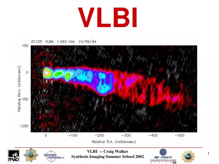
VLBI VLBI -- Craig Walker Synthesis Imaging Summer School 2002
What is VLBI?(Very Long Baseline Interferometry) • Radio interferometry with unlimited baselines • For high resolution – milliarcsecond (mas) or better • Baselines up to an Earth diameter for ground based VLBI • Can extend to space (HALCA) • Traditionally uses no IF or LO link between antennas • Atomic clocks for time and frequency– usually hydrogen masers • Tape recorders for data transmission • Disk based systems under development • Delayed correlation after tapes shipped • Real time over fiber is a long term goal • Can use antennas built for other reasons • Not fundamentally different from linked interferometry VLBI -- Craig Walker Synthesis Imaging Summer School 2002
THE QUEST FOR RESOLUTION Atmosphere gives 1" limit without corrections which are easiest in radio Jupiter and Io as seen from Earth 1 arcmin 1 arcsec 0.05 arcsec 0.001 arcsec Simulated with Galileo photo
Brightness Temperature Sensitivity Tb sensitivity = Tbs Filling Factor Tbs = Tb sensitivity of equivalent area single dish Filling factor 1/D2 so VLBI can only see very “Bright” sources Independent of frequency Density of sources much greater at low flux density
GLOBAL VLBI STATIONS Geodesy stations. Some astronomy stations missing, especially in Europe. VLBI -- Craig Walker Synthesis Imaging Summer School 2002
The VLBA Ten 25m Antennas, 20 Station Correlator 327 MHz - 86 GHz National Radio Astronomy Observatory A Facility of the National Science Foundation
VLBI SCIENCE SAMPLES CAPABILITY EXAMPLE SCIENCE Jet formation Jet dynamics and magnetic fields Detect survey sources, distinguish starbursts from AGN Accurate proper motions Accretion disks and extra galactic distances Stellar environments Plate motions, EOP, reference frames High resolution continuum Movies and polarization Phase referencing to detect weak sources Phase referencing for positions High resolution spectral line Spectral line movies Geodesy and astrometry VLBI -- Craig Walker Synthesis Imaging Summer School 2002
M87 Inner Jet M87 Base of Jet 43 GHz Global VLBI Junor, Biretta, & Livio Nature, 401, 891 VLA Images Resolution 0.000330.00012 Black Hole / Jet Model VLBI Image
3C120 43 GHz VLBA Movie Gómez et al. Science 289, 2317 Bottom: Contours of intensity Color shows polarized flux Top: Color shows intensity Lines show B vectors Resolution ~0."0005 One image / Month Intensity and polarization variations suggest jet-cloud interaction Between 2 and 4 mas from core (~8 pc) Cloud would be intermediate in mass between broad and narrow line clouds.
AGN or Starburst?Weak source detection Would like to distinguish AGN from starbursts in surveys etc. Starburst will have brightness temperature too low to detect VLBI detection implies it is an AGN Example from VLBA+EB+GBT Phase referencing 1.4 GHz Peak 104 Jy. Total 1.2 mJy RMS noise 10 Jy From Fomalont (survey observations) VLBI -- Craig Walker Synthesis Imaging Summer School 2002
MOTIONS OF SGRA* Measures rotation of the Milky Way Galaxy 0.00590.4 / yr Reid et al. 1999, Ap. J. 524, 816 VLBI -- Craig Walker Synthesis Imaging Summer School 2002
H2O masers in edge-on accretion disk Clear Keplerian rotation Orbit speed from Doppler shifts of masers Central mass from orbit speed and radius Distance from transverse angular motion or acceleration of central masers The Black Hole in NGC 4258 Central mass = 3.6 107 solar mass (Miyoshi et al. Nature 373, 127) Distance = 7.2 0.3 0.5 Mpc (Herrnstein et al. Nature 400, 539)
SiO Masers in TX Cam Mira variable (Pulsating star) VLBA 43 GHz, two week intervals Full velocity and polarization information available Diamond and Kemball
GEODESY and ASTROMETRY • Fundamental reference frames • International Celestial Reference Frame (ICRF) • International Terrestrial Reference Frame (ITRF) • Earth rotation and orientation relative to inertial reference frame of distant quasars • Tectonic plate motions measured directly • Earth orientation data used in studies of Earth’s core and Earth/atmosphere interaction • General relativity tests • Solar bending significant over whole sky VLBI -- Craig Walker Synthesis Imaging Summer School 2002
PLATE MOTIONSGERMANY to MASSACHUSETTS Note improvement of errors over time Plate motion is clear Possible annual effects starting to show From GSFC VLBI group - Jan 2000 solution 10 cm Baseline Length 1984-1999 Baseline transverse 10 cm
DATA REDUCTIONVLBI vs LINKED INTERFEROMETRY VLBI is not fundamentally different from linked interferometry Differences are a matter of degree Separate clocks allow rapid changes in instrumental phase Independent atmospheres give rapid phase variations and large gradients Different source elevations exacerbate the effect Sources bright enough to be both easily detectable and compact to VLBI are small, highly energetic, and variable There are no flux calibrators There are no polarization position angle calibrators There are no good point source amplitude calibrators Model uncertainties are can be large Source positions, station locations, and the Earth orientation are difficult to determine to a small fraction of a wavelength Often use antennas not designed for interferometry. Not very phase stable VLBI -- Craig Walker Synthesis Imaging Summer School 2002
VLBI Data ReductionUnique Aspects • Schedule fringe finder observations (Helps correlator operations) • Correct instrumental phases with pulse calibration tones • Correct high delay and phase rate offsets with fringe fit • Phase referencing requires short throws and fast cycles • Calibrate flux density using telescope a priori gains • Calibrate polarization PA using near concurrent observations on a short baseline instrument • Image calibrators • Strong source imaging usually based on self calibration with very poor starting model VLBI -- Craig Walker Synthesis Imaging Summer School 2002
VLBA Station Electronics At antenna: Select RCP and LCP Add calibration signals Amplify Mix to IF (500-1000 MHz) In building: Distribute to baseband converters (8) Mix to baseband Filter (0.062 - 16 MHz) Sample (1 or 2 bit) Format for tape (32 track) Record Also keep time and stable frequency Other systems conceptually similar VLBA STATION ELECTRONICS
JIVE Correlator VLBICORRELATOR • Read tapes • Synchronize data • Apply delay model (includes phase model ) • Correct for known Doppler shifts (Mainly from Earth rotation) • This is the total fringe rate and is related to the rate of change of delay • FX: FFT then cross multiply spectra (VLBA) • XF: Cross multiply lags. FFT later (JIVE, Haystack, VLA …) • Accumulate and write data to archive • Some corrections may be required in postprocessing • Data normalization and scaling (Varies by correlator) • Corrections for clipper offsets (ACCOR in AIPS) VLBI -- Craig Walker Synthesis Imaging Summer School 2002
THE DELAY MODEL For 8000 km baseline 1 mas = 3.9 cm = 130 ps Adapted from Sovers, Fanselow, and Jacobs Reviews of Modern Physics, Oct 1998
Raw Residual Data from Correlator • Significant phase changes with time (fringe rates) • Significant phase slopes in frequency (delays) • Can contain bad data, although that not shown in this example VLBI -- Craig Walker Synthesis Imaging Summer School 2002
VLBI Amplitude Calibration • Scij = Correlated flux density on baseline i - j • = Measured correlation coefficient • A = Correlator specific scaling factor • s= System efficiency including digitization losses • Ts = System temperature • Includes receiver, spillover, atmosphere, blockage • K = Gain in degrees K per Jansky • Includes gain curve • e- = Absorption in atmosphere plus blockage • Note Ts/K = SEFD (System Equivalent Flux Density) VLBI -- Craig Walker Synthesis Imaging Summer School 2002
Calbration with Tsys Example shows removal of effect of increased Ts due to rain and low elevation
Atmospheric opacity Correcting for absorption by the atmosphere Can estimate using Ts – Tr – Tspill Example from single-dish VLBA pointing data Gain curves and Opacity correction VLBA gain curves Caused by gravity induced distortions of the antenna as a function of elevation
Pulse Cal System Tones generated by injecting pulse once per microsecond Use to correct for instrumental phase shifts pcal tones Cable Cal Pulse Cal Monitor data 50 ps A Long Track Data Aligned with Pulse Cal A 10 ps Geodesy – Long Slews At c, 1 ps = 3mm A No PCAL at VLA Shows unaligned phases Long track at non-VLBA station
Ionospheric Delay • Delay scales with 1/2 • Ionosphere dominates errors at low frequencies • Can correct with dual band observations (S/X) • GPS based ionosphere models help (AIPS task TECOR) Maximum Likely Ionospheric Contributions Ionosphere map from iono.jpl.nasa.gov Delays from an S/X Geodesy Observation -20 Delay (ns) 20 8.4 GHz2.3 GHz Time (Days)
Raw Data - No Edits EDITING A (Jy) (deg) A (Jy) (deg) • Flags from on-line system will remove most bad data • Antenna off source • Subreflector out of position • Synthesizers not locked • Final flagging done by examining data • Best to flag antennas - nearly all causes of poor data are antenna based • Poor weather • Bad playback • RFI (May need to flag by channel) • On-line flags not perfect Raw Data - Edited A (Jy) (deg) A (Jy) (deg)
Bandpass Calibration • Based on bandpass calibration source • Effectively a self-cal on a per-channel basis • Needed for spectral line calibration • May help continuum calibration by reducing closure errors • Affected by high total fringe rates • Fringe rate shifts spectrum relative to filters • Bandpass spectra must be shifted to align filters when applied • Will lose edge channels in process of correcting for this. Before After
Typical calibrator visibility function after a priori calibration but before fine tuning with model Amplitude Check Source Resolved – a model or image will be needed Poorly calibrated antenna
FRINGE FITTING: WHAT and WHY • Raw correlator output has phase slopes in time and frequency • Slope in time is “fringe rate” • Fluctuations worse at high frequency because of water vapor • Slope in frequency is “delay” (from ) • Fluctuations worse at low frequency because of ionosphere • Fringe fit is self calibration with first derivatives in time and frequency • For Astronomy: • Fit one or a few scans to “set clocks” and align channels (“manual pcal”) • Fit calibrator to track most variations (optional) • Fit target source if strong (optional) • Used to allow averaging in frequency and time • Used to allow higher SNR self calibration (longer solution) • Allows corrections for smearing from previous averaging • For geodesy • Fitted delays are the primary “observable” • Slopes fitted over wide frequency range (“Bandwidth Synthesis”) • Correlator model is added to get “total delay” VLBI -- Craig Walker Synthesis Imaging Summer School 2002
FRINGE FITTING: HOW • Usually a two step process • 2D FFT to get estimated rates and delays to reference antenna • Required for start model for least squares • Can restrict window to avoid high sigma noise points • Can use just baselines to reference antenna or can stack 2 and even 3 baseline combinations • Least squares fit to phases starting at FFT estimate • Baseline fringe fit • Not affected by poor source model • Used for geodesy. Noise more accountable. • Global fringe fit (like self cal) • One phase, rate, and delay per antenna • Best SNR because all data used • Improved by good source model • Best for imaging VLBI -- Craig Walker Synthesis Imaging Summer School 2002
Movies made by George Moellenbrock using AIPS++ FRINGE FITTING EXAMPLE: HIGH SNR CASE Result of fringe fit FFT (Amplitude of transform) Source is easily seen in one integration time / frequency channel Input Phases (several turns) Fringe Rate Time Delay Frequency VLBI -- Craig Walker Synthesis Imaging Summer School 2002
Movies made by George Moellenbrock using AIPS++ FRINGE FITTING EXAMPLE: LOW SNR CASE Result of fringe fit FFT (Amplitude of transform) Source cannot be seen in one integration time / frequency channel Input Phases (several turns) Fringe Rate Time Delay Frequency VLBI -- Craig Walker Synthesis Imaging Summer School 2002
Self Calibration Imaging • Can image even if calibration is poor or nonexistent • Possible because there are N gains and N(N-2)/2 baselines • Can determine both source structure and antenna gains • Need at least 3 antennas for phase gains, 4 for amplitude gains • Works better with many antennas • Iterative procedure: • Use best available image to solve for gains (can start with point) • Use gains to derive improved image • Should converge quickly for simple sources • Many iterations (~50-100) may be needed for complex sources • May need to vary some imaging parameters between iterations • Should reach near thermal noise in most cases • Does not preserve absolute position or flux density scale • Gain normalization usually makes this problem minor • Historically called “Hybrid Mapping”. Based on “Closure Phase”. • Is required for highest dynamic ranges on all interferometers VLBI -- Craig Walker Synthesis Imaging Summer School 2002
Example Self Cal Imaging Sequence • Start with phase only selfcal • Add amplitude cal when progress slows • Vary parameters between iterations • Taper, robustness, uvrange etc • Try to reach thermal noise • Should get close
PHASE REFERENCING • Use phase calibrator outside target source field • Nodding calibrator (move antennas) • In-beam calibrator (separate correlation pass) • Multiple calibrators for most accurate results • Very similar to VLA calibration but: • Geometric and atmospheric models worse • Affected by totals between antennas, not just differentials • Model errors usually dominate over fluctuations • Scale with total error times source-target separation in radians • Need to calibrate often (5 minute or faster cycle) • Need calibrator close to target (< 5 deg) • Biggest problems: • Wet troposphere at high frequency • Ionosphere at low frequencies (20 cm is as bad as 1cm) • Use for weak sources and for position measurements • Increases sensitivity by 1 to 2 orders of magnitude • Used by about 30-50% of VLBA observations
EXAMPLE OF REFERENCED PHASES • 6 min cycle - 3 on each source • Phases of one source self-calibrated (near zero) • Other source shifted by same amount VLBI -- Craig Walker Synthesis Imaging Summer School 2002
Phase Referencing Example • With no phase calibration, source is not detected (no surprise) • With reference calibration, source is detected, but structure is distorted (target-calibrator separation is probably not small) • Self-calibration of this strong source shows real structure No Phase Calibration Reference Calibration Self-calibration
GEODETIC and ASTROMETRIC OBSERVATIONS • Use group delays from wide spanned bandwidths • Use “totals” with correlator model added back in • Use 2.3 and 8.4 GHz (S/X) to remove ionosphere • Can do global fits to all historical geodesy data • Fits include: • Antenna and source positions • Earth orientation (UT1-UTC, nutation, …) • Time variable atmosphere and clocks • Many other possible parameters • Accuracy is better than 1 mas for source position and 1cm for antenna positions • Observing by service groups, often using dedicated antennas VLBI -- Craig Walker Synthesis Imaging Summer School 2002
SCHEDULING • PI provides detailed observation sequence • Include fringe finders (strong sources - at least 2 scans) • Include amplitude check source (compact source) • If target weak, include a delay/rate calibrator • If target very weak, fast switch to a phase calibrator • For spectral line observations, include bandpass calibrator • For polarization observations, include polarization calibrators • Get good paralactic angle coverage on one to get instrumental terms • Observe absolute position angle calibrator • Leave occasional gaps for tape readback tests (2 min) • For non-VLBA observations, manage tapes (passes and changes) VLBI -- Craig Walker Synthesis Imaging Summer School 2002
FUTURE DEVELOPMENT • Use GPS tropospheric delays for calibration • Use water vapor radiometers for calibration • Use improved ionosphere models when available (especially 3D) • Regular use of multi-frequency synthesis (MFS) • Use pulse cal for Tsys measurement; for polarization PA calibration • Push to higher frequencies • More use of large antennas (GBT, EB, Arecibo, Y27) • Develop robust automated imaging procedures • Technical push to wider bandwidths and real time • Fill in shorter baselines • MERLIN/VLBI integration in Europe; EVLA/VLBA integration in US • Future space projects • Big sensitivity increase with long baselines of SKA VLBI -- Craig Walker Synthesis Imaging Summer School 2002
THE END VLBI -- Craig Walker Synthesis Imaging Summer School 2002