Download
1 / 18
180 likes | 186 Views
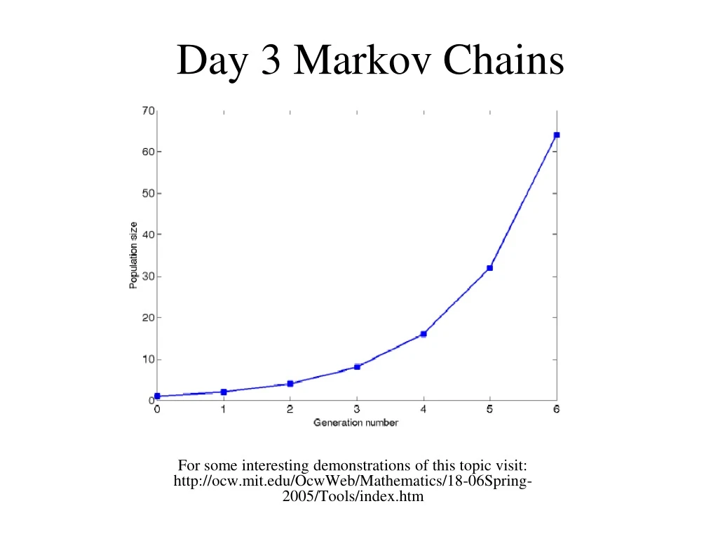
Day 3 Markov Chains. For some interesting demonstrations of this topic visit: http:// ocw.mit.edu / OcwWeb /Mathematics/18-06Spring-2005/Tools/ index.htm. Equations of the form: are called discrete equations because they only model the system at whole number time increments.

E N D
Day 3 Markov Chains For some interesting demonstrations of this topic visit: http://ocw.mit.edu/OcwWeb/Mathematics/18-06Spring-2005/Tools/index.htm
Equations of the form:are called discrete equations because they only model the system at whole number time increments. • Difference equation is an equation involving differences. We can see difference equation from at least three points of views: as sequence of number, discrete dynamical system and iterated function. It is the same thing but we look at different angle.
Difference Equations vs. Differential Equations Dynamical system come with many different names. Our particular interesting dynamical system is for the system whose state depends on the input history. In discrete time system, we call such system difference equation (equivalent to differential equation in continuous time).
Markov Matrices Consider the matrix Properties of Markov Matrices: All entries are ≥ 0. All Columns add up to one. Note: the powers of the matrix will maintain these properties. Each column is representing probabilities.
Markov Matrices 1 is an eigenvalue of all Markov Matrices Why? Subtract 1 down each entry in the diagonal. Each column will then add to zero - which means that the rows are dependent. - which means that the matrix is singular.
[ ] Markov Matrices 0.1 0.01 0.3 A = 0.2 0.99 0.3 0.7 0 0.4 One eigenvalue is 1 all other eigenvalues have an absolute value ≤ 1. We are interested in raising A to some powers If 1 is an eigenvector and all other vectors are less than 1 then the steady state is the eigenvector. Note: this requires n independent vectors.
[ ] Short cuts for finding eigenvectors -0.9 0.01 0.3 A - I = 0.2 -0.01 0.3 det ( A -1I ) 0.7 0 -0.6 To find the eigenvector that corresponds to λ = 1 Use to get the last row to be zero. Then use the top row to get the missing middle value. (working on next slide)
Short cuts for finding eigenvectors Then use the top row to get the missing middle value. (-0.9)(0.6) + (0.01)(???) + (0.3)(0.7) = 0 ??? = 33 Or the 2nd row to get the middle value (0.2)(0.6) + (-0.01)(???) + (0.3)(0.7) = 0 ??? = 33
Applications of Markov Matrices Markov Matrices are used to when the probability of an event depends on its current state. For this model, the probability of an event must remain constant over time. The total population is not changing over time. Markov matrices have applications in Electrical engineering, waiting times, stochastic process.
Applications of Markov Matrices uk+1 = Auk Suppose we have two cities Suzhou (S) and Hangzhou (H) with initial condition at k = 0, S = 0 and H =1000. We would like to describe movement in population between these two cities. us+1 =0.9 0.2 uS uH+1 0.1 0.8 uH Population of Suzhou and Hongzhou at time t+1 Column 1: .9 of the people in S stay there and .1 move to H Column 2: .8 of the people in H stay there are and .2 move to S [ ] [ ] [ ] Population of S and H at time t
Applications of Markov Matrices current state [ ] [ ] [ ] [ ] uk+1 = Auk us+1 = 0 .9 0.2 uS uH +1 0.1 0.8 uH Find the eigenvalues and eigenvectors. next state
Applications of Markov Matrices [ ] [ ] [ ] uk+1 = Auk us+1 = 0 .9 0.2 uS uH +1 0.1 0.8 uH Find the eigenvalues and eigenvectors. Eigenvalues: λ1 = 1 and λ2 = 0.7 (from properties of Markov Matrices and the trace) Eigenvectors: ker (A - I) , ker (A - 0.7I)
Applications of Markov Matrices [ ] [ ] [ ] uk+1 = Auk us+1 = 0 .9 0.2 uS uH +1 0.1 0.8 uH eigenvalue 1 eigenvalue 0.7 eigenvector eigenvector This tells us about time and ∞. λ = 1 will be a steady state, λ = 0.7 will disappear as t → ∞ The eigenvector tells us that we need a ratio of 2:1. The total population is still 1000 so the final population will be 1000 (2/3) and 1000 (1/3).
Initial condition at k=0, S = 0 and H = 1000 Applications [ ] [ ] [ ] us+1 = .9 .2 uS uH +1 .1 .8 uH To find the amounts after a finite number of steps Aku0 = c1(1)k 2 + c2(0.7)k -1 1 1 Use the initial condition to solve for constants 0 = c1 2 + c2 -1 c1 = 1000/3 1000 1 1 c2 = 2000/3 [ ] [ ] [ ] [ ] [ ]
Steady state for Markov Matrices Every Markov chain will be a steady state. The steady state will be the eigenvector for the eigenvalue λ = 1.
Homework: p. 487 3-6,8,9,13 white book, eigenvalue review worksheet 1-5 "Genius is one per cent inspiration, ninety-nine per cent perspiration.“ Thomas Alva Edison
More Info http://ocw.mit.edu/courses/mathematics/18-06-linear-algebra-spring-2010/video-lectures/lecture-24-markov-matrices-fourier-series/ www.math.hawaii.edu/~pavel/fibonacci.pdf http://people.revoledu.com/kardi/tutorial/DifferenceEquation/WhatIsDifferenceEquation.htm https://www.math.duke.edu//education/ccp/materials/linalg/diffeqs/diffeq2.html
For More information visit: Fibonacci via matrices http://www.maths.leeds.ac.uk/applied/0380/fibonacci03.pdf