Download

1 / 34
340 likes | 380 Views
Integrals. 5. Approximate Integration. 5.9. Approximate Integration. There are two situations in which it is impossible to find the exact value of a definite integral.

E N D
Approximate Integration • There are two situations in which it is impossible to find the exact value of a definite integral. • The first situation arises from the fact that in order to evaluate using the Evaluation Theorem we need to know an antiderivative of f. • Sometimes, however, it is difficult, or even impossible, to find an antiderivative. For example, it is impossible to evaluate the following integrals exactly:
Approximate Integration • The second situation arises when the function is determined from a scientific experiment through instrument readings or collected data. • There may be no formula for the function. • In both cases we need to find approximate values of definite integrals. We already know one such method.
Approximate Integration • Recall that the definite integral is defined as a limit of Riemann sums, so any Riemann sum could be used as an approximation to the integral: If we divide [a, b] into n subintervals of equal length x = (b – a)/n,then we have • where xi* is any point in the ith subinterval [xi–1, xi]. If xi* is chosen to be the left endpoint of the interval, then xi* = xi–1 and we have
Approximate Integration • If f(x) 0, then the integral represents an area and (1) represents an approximation of this area by the rectangles shown in Figure 1(a) with n = 4. Figure 1(a)
Approximate Integration • If we choose xi* to be the right endpoint, then xi* = xi and we have • [See Figure 1(b).] • The approximations Ln and Rndefined by Equations 1 and 2 are called the left endpoint approximation and right endpoint • approximation, respectively. Figure 1(b)
Approximate Integration • We also considered the case where xi* is chosen to be the midpoint of the subinterval [xi–1, xi]. Figure 1(c) shows the midpoint approximation Mn, which appears to be better than either Ln or Rn. Figure 1(c)
Approximate Integration • Another approximation, called the Trapezoidal Rule, results from averaging the approximations in Equations 1 and 2:
Approximate Integration • The reason for the name Trapezoidal Rule can be seen from Figure 2, which illustrates the case with f(x) 0 and n = 4. Figure 2 Trapezoidal approximation
Approximate Integration • The area of the trapezoid that lies above the ith subinterval is • and if we add the areas of all these trapezoids, we get the right side of the Trapezoidal Rule.
Example 1 • Use (a) the Trapezoidal Rule and (b) the Midpoint Rule with • n = 5 to approximate the integral • Solution: • (a) With n = 5, a = 1 and b = 2, we have x =(2 – 1)/5 = 0.2, • and so the Trapezoidal Rule gives • ≈ 0.695635
Example 1 – Solution cont’d • This approximation is illustrated in Figure 3. Figure 3
Example 1 – Solution cont’d • (b) The midpoints of the five subintervals are 1.1, 1.3, 1.5, • 1.7, and 1.9, so the Midpoint Rule gives • ≈ 0.691908 • This approximation is • illustrated in Figure 4. Figure 4
Approximate Integration • In Example 1 we deliberately chose an integral whose value can be computed explicitly so that we can see how accurate the Trapezoidal and Midpoint Rules are. • By the fundamental Theorem of Calculus, • The error in using an approximation is defined to be the amount that needs to be added to the approximation to make it exact.
Approximate Integration • From the values in Example 1 we see that the errors in the Trapezoidal and Midpoint Rule approximations for n = 5 are • ET≈ –0.002488 and EM ≈ 0.001239 • In general, we have
Approximate Integration • The following tables show the results of calculations similar to those in Example 1, but for n = 5, 10, and 20 and for the left and right endpoint approximations as well as the Trapezoidal and Midpoint Rules.
Approximate Integration • We can make several observations from these tables: • 1. In all of the methods we get more accurate approximations when we increase the value of n. (But very large values of n result in so many arithmetic operations that we have to beware of accumulated round-off error.) • 2. The errors in the left and right endpoint approximations are opposite in sign and appear to decrease by a factor of about 2 when we double the value of n.
Approximate Integration • 3. The Trapezoidal and Midpoint Rules are much more accurate than the endpoint approximations. • 4. The errors in the Trapezoidal and Midpoint Rules are opposite in sign and appear to decrease by a factor of about 4 when we double the value of n. • 5. The size of the error in the Midpoint Rule is about half the size of the error in the Trapezoidal Rule.
Approximate Integration • Let’s apply this error estimate to the Trapezoidal Rule approximation in Example 1. • If f(x) = 1/x, then f(x) = –1/x2 and f(x) = 2/x3.
Approximate Integration • Since 1 x 2, we have 1/x 1, so • Therefore, taking K = 2, a = 1, b = 2, and n = 5 in the error estimate (3), we see that • Comparing this error estimate of 0.006667 with the actual error of about 0.002488, we see that it can happen that the actual error is substantially less than the upper bound for theerror given by (3).
Simpson’s Rule • Another rule for approximate integration results from using parabolas instead of straight line segments to approximate a curve. • As before, we divide [a, b] into n subintervals of equal length h = x =(b – a)/n, but this time we assume that n is an even number.
Simpson’s Rule • Then on each consecutive pair of intervals we approximate the curve y = f(x) 0 by a parabola as shown in Figure 7. • If yi = f(xi), then Pi(xi, yi) is the point on the curve lying • above xi. Figure 7
Simpson’s Rule • A typical parabola passes through three consecutive points Pi , Pi+1, and Pi+2. • To simplify our calculations, we first consider the case where x0 = –h, x1 = 0, and x2 = h. (See Figure 8.) Figure 8
Simpson’s Rule • We know that the equation of the parabola through P0, P1,and P2is of the form y = Ax2 + Bx + C and so the area under the parabola from x = –h to x = h is
Simpson’s Rule • But, since the parabola passes through P0(–h, y0), P1(0, y1), and P2(h, y2), we have • y0 = A(–h)2 + B(–h) + C = Ah2 – Bh + C • y1 = C • y2 = Ah2 + Bh + C • and therefore y0 +4y1 + y2 = 2Ah2 + 6C • Thus we can rewrite the area under the parabola as • (y0 +4y1 + y2)
Simpson’s Rule • Now, by shifting this parabola horizontally we do not change the area under it. • This means that the area under the parabola through P0, P1, and P2 from x = x0 to x = x2 in Figure 7 is still • (y0 +4y1 + y2) Figure 7
Simpson’s Rule • Similarly, the area under the parabola through P2, P3,and P4 from x = x2 to x = x4 is • (y2 +4y3 + y4) • If we compute the areas under all the parabolas in this manner and add the results, we get
Simpson’s Rule • Although we have derived this approximation for the case in which f(x) 0, it is a reasonable approximation for any continuous function f and is called Simpson’s Rule after the English mathematician Thomas Simpson (1710–1761). • Note the pattern of coefficients: • 1, 4, 2, 4, 2, 4, 2, . . . , 4, 2, 4, 1.
Example 4 • Use Simpson’s Rule with n = 10 to approximate • Solution: • Putting f(x) = 1/x, n = 10, and x = 0.1 in Simpson’s Rule, we obtain
Simpson’s Rule • The Trapezoidal Rule or Simpson’s Rule can still be used to find an approximate value for the integral of y with respect to x. • The table below shows how Simpson’s Rule compares with the Midpoint Rule for the integral whose true value is about 0.69314718. • The second table shows how the error Esin Simpson’s Rule decreases by a factor of about 16 when n is doubled.
Simpson’s Rule • That is consistent with the appearance of n4 in the denominator of the following error estimate for Simpson’s Rule. • It is similar to the estimates given in (3) for the Trapezoidal and Midpoint Rules, but it uses the fourth derivative of f.