Download
1 / 69
690 likes | 701 Views
Statistical Methods for Particle Physics Lecture 2: Introduction to Multivariate Methods. www.pp.rhul.ac.uk/~cowan/stat_trisep.html. Lectures on Statistics TRISEP School 27, 28 June 2016. Glen Cowan Physics Department Royal Holloway, University of London g.cowan@rhul.ac.uk

E N D
Statistical Methods for Particle PhysicsLecture 2: Introduction to Multivariate Methods www.pp.rhul.ac.uk/~cowan/stat_trisep.html Lectures on Statistics TRISEP School 27, 28 June 2016 Glen Cowan Physics Department Royal Holloway, University of London g.cowan@rhul.ac.uk www.pp.rhul.ac.uk/~cowan TRISEP 2016 / Statistics Lecture 2 TexPoint fonts used in EMF. Read the TexPoint manual before you delete this box.: AAAA
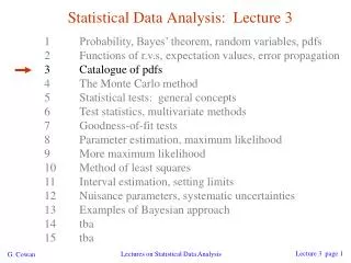
Outline Lecture 1: Introduction and review of fundamentals Probability, random variables, pdfs Parameter estimation, maximum likelihood Statistical tests for discovery and limits Lecture 2: Multivariate methods Neyman-Pearson lemma Fisher discriminant, neural networks Boosted decision trees Lecture 3: Systematic uncertainties and further topics Nuisance parameters (Bayesian and frequentist) Experimental sensitivity The look-elsewhere effect TRISEP 2016 / Statistics Lecture 2
Resources on multivariate methods C.M. Bishop, Pattern Recognition and Machine Learning, Springer, 2006 T. Hastie, R. Tibshirani, J. Friedman, The Elements of Statistical Learning, 2nd ed., Springer, 2009 R. Duda, P. Hart, D. Stork, Pattern Classification, 2nd ed., Wiley, 2001 A. Webb, Statistical Pattern Recognition, 2nd ed., Wiley, 2002. Ilya Narsky and Frank C. Porter, Statistical Analysis Techniques in Particle Physics, Wiley, 2014. 朱永生(编著),实验数据多元统计分析,科学出版社,北京,2009。 TRISEP 2016 / Statistics Lecture 2
Software Rapidly growing area of development – two important resources: TMVA, Höcker, Stelzer, Tegenfeldt, Voss, Voss, physics/0703039 From tmva.sourceforge.net, also distributed with ROOT Variety of classifiers Good manual, widely used in HEP scikit-learn Python-based tools for Machine Learning scikit-learn.org Large user community TRISEP 2016 / Statistics Lecture 2
A simulated SUSY event in ATLAS high pT jets of hadrons high pT muons p p missing transverse energy TRISEP 2016 / Statistics Lecture 2
Background events This event from Standard Model ttbar production also has high pT jets and muons, and some missing transverse energy. → can easily mimic a SUSY event. TRISEP 2016 / Statistics Lecture 2
Defining a multivariate critical region For each event, measure, e.g., x1 = missing energy, x2 = electron pT, x3 = ... Each event is a point in n-dimensional x-space; critical region is now defined by a ‘decision boundary’ in this space. What is best way to determine the boundary? H0 (b) Perhaps with ‘cuts’: H1 (s) W TRISEP 2016 / Statistics Lecture 2
Other multivariate decision boundaries Or maybe use some other sort of decision boundary: linear or nonlinear H0 H0 H1 H1 W W Multivariate methods for finding optimal critical region have become a Big Industry (neural networks, boosted decision trees,...), benefitting from recent advances in Machine Learning. TRISEP 2016 / Statistics Lecture 2
Test statistics The boundary of the critical region for an n-dimensional data space x = (x1,..., xn) can be defined by an equation of the form where t(x1,…, xn) is a scalar test statistic. We can work out the pdfs Decision boundary is now a single ‘cut’ on t, defining the critical region. So for an n-dimensional problem we have a corresponding 1-d problem. TRISEP 2016 / Statistics Lecture 2
Test statistic based on likelihood ratio How can we choose a test’s critical region in an ‘optimal way’? Neyman-Pearson lemma states: To get the highest power for a given significance level in a test of H0, (background) versus H1, (signal) the critical region should have inside the region, and ≤ c outside, where c is a constant chosen to give a test of the desired size. Equivalently, optimal scalar test statistic is N.B. any monotonic function of this is leads to the same test. TRISEP 2016 / Statistics Lecture 2
Neyman-Pearson doesn’t usually help We usually don’t have explicit formulae for the pdfs f(x|s), f(x|b), so for a given x we can’t evaluate the likelihood ratio Instead we may have Monte Carlo models for signal and background processes, so we can produce simulated data: generate x ~ f(x|s) → x1,..., xN generate x ~ f(x|b) → x1,..., xN This gives samples of “training data” with events of known type. Can be expensive (1 fully simulated LHC event ~ 1 CPU minute). TRISEP 2016 / Statistics Lecture 2
Approximate LR from histograms Want t(x) = f(x|s)/f(x|b) for x here One possibility is to generate MC data and construct histograms for both signal and background. Use (normalized) histogram values to approximate LR: N(x|s) N(x|s) ≈ f(x|s) x N(x|b) N(x|b) ≈ f(x|b) Can work well for single variable. x TRISEP 2016 / Statistics Lecture 2
Approximate LR from 2D-histograms Suppose problem has 2 variables. Try using 2-D histograms: back- ground signal Approximate pdfs using N(x,y|s), N(x,y|b) in corresponding cells. But if we want M bins for each variable, then in n-dimensions we have Mn cells; can’t generate enough training data to populate. →Histogram method usually not usable for n > 1 dimension. TRISEP 2016 / Statistics Lecture 2
Strategies for multivariate analysis Neyman-Pearson lemma gives optimal answer, but cannot be used directly, because we usually don’t have f(x|s), f(x|b). Histogram method with M bins for n variables requires that we estimate Mn parameters (the values of the pdfs in each cell), so this is rarely practical. A compromise solution is to assume a certain functional form for the test statistic t(x) with fewer parameters; determine them (using MC) to give best separation between signal and background. Alternatively, try to estimate the probability densities f(x|s) and f(x|b) (with something better than histograms) and use the estimated pdfs to construct an approximate likelihood ratio. TRISEP 2016 / Statistics Lecture 2
Linear test statistic Suppose there are n input variables: x = (x1,..., xn). Consider a linear function: For a given choice of the coefficients w = (w1,..., wn) we will get pdfs f(y|s) and f(y|b) : TRISEP 2016 / Statistics Lecture 2
Linear test statistic Fisher: to get large difference between means and small widths for f(y|s) and f(y|b), maximize the difference squared of the expectation values divided by the sum of the variances: Setting ∂J/∂wi = 0 gives for w = (w1, ... wn): , TRISEP 2016 / Statistics Lecture 2
The Fisher discriminant The resulting coefficients wi define a Fisher discriminant. Coefficients defined up to multiplicative constant; can also add arbitrary offset, i.e., usually define test statistic as Boundaries of the test’s critical region are surfaces of constant y(x), here linear (hyperplanes): TRISEP 2016 / Statistics Lecture 2
Fisher discriminant for Gaussian data Suppose the pdfs of the input variables, f(x|s) and f(x|b), are both multivariate Gaussians with same covariance but different means: f(x|s) = Gauss(μs, V) Same covariance Vij = cov[xi, xj] f(x|b) = Gauss(μb, V) In this case it can be shown that the Fisher discriminant is i.e., it is a monotonic function of the likelihood ratio and thus leads to the same critical region. So in this case the Fisher discriminant provides an optimal statistical test. TRISEP 2016 / Statistics Lecture 2
The activation function For activation function h(·) often use logistic sigmoid: TRISEP 2016 / Statistics Lecture 2
Network architecture Theorem: An MLP with a single hidden layer having a sufficiently large number of nodes can approximate arbitrarily well the optimal decision boundary. Holds for any continuous non-polynomial activation function Leshno, Lin, Pinkus and Schocken (1993) Neural Networks 6, 861-867 However, the number of required nodes may be very large; cannot train well with finite samples of training data. Recent advances in Deep Neural Networks have shown important advantages in having multiple hidden layers. For a particle physics application of Deep Learning, see e.g. Baldi, Sadowski and Whiteson, Nature Communications 5 (2014); arXiv:1402.4735. TRISEP 2016 / Statistics Lecture 2
Overtraining Including more parameters in a classifier makes its decision boundary increasingly flexible, e.g., more nodes/layers for a neural network. A “flexible” classifier may conform too closely to the training points; the same boundary will not perform well on an independent test data sample (→“overtraining”). independent test sample training sample TRISEP 2016 / Statistics Lecture 2
Monitoring overtraining If we monitor the fraction of misclassified events (or similar, e.g., error function E(w)) for test and training samples, it will usually decrease for both as the boundary is made more flexible: optimum at minimum of error rate for test sample error rate increase in error rate indicates overtraining test sample training sample flexibility (e.g., number of nodes/layers in MLP) TRISEP 2016 / Statistics Lecture 2
Neural network example from LEP II Signal: e+e-→ W+W- (often 4 well separated hadron jets) Background: e+e-→ qqgg (4 less well separated hadron jets) ← input variables based on jet structure, event shape, ... none by itself gives much separation. Neural network output: (Garrido, Juste and Martinez, ALEPH 96-144) TRISEP 2016 / Statistics Lecture 2
Each event characterized by 3 variables, x, y, z: TRISEP 2016 / Statistics Lecture 2
Test example (x, y, z) y y no cut on z z < 0.75 x x y y z < 0.25 z < 0.5 x x TRISEP 2016 / Statistics Lecture 2
Test example results Fisher discriminant Multilayer perceptron Naive Bayes, no decor- relation Naive Bayes with decor- relation TRISEP 2016 / Statistics Lecture 2
Particle i.d. in MiniBooNE Detector is a 12-m diameter tank of mineral oil exposed to a beam of neutrinos and viewed by 1520 photomultiplier tubes: Search for νμ to νe oscillations required particle i.d. using information from the PMTs. H.J. Yang, MiniBooNE PID, DNP06 TRISEP 2016 / Statistics Lecture 2
Decision trees Out of all the input variables, find the one for which with a single cut gives best improvement in signal purity: where wi. is the weight of the ith event. Resulting nodes classified as either signal/background. Iterate until stop criterion reached based on e.g. purity or minimum number of events in a node. The set of cuts defines the decision boundary. Example by MiniBooNE experiment, B. Roe et al., NIM 543 (2005) 577 TRISEP 2016 / Statistics Lecture 2
Finding the best single cut The level of separation within a node can, e.g., be quantified by the Gini coefficient, calculated from the (s or b) purity as: For a cut that splits a set of events a into subsets b and c, one can quantify the improvement in separation by the change in weighted Gini coefficients: where, e.g., Choose e.g. the cut to the maximize Δ; a variant of this scheme can use instead of Gini e.g. the misclassification rate: TRISEP 2016 / Statistics Lecture 2
Decision tree classifier The terminal nodes (leaves) are classified a signal or background depending on majority vote (or e.g. signal fraction greater than a specified threshold). This classifies every point in input-variable space as either signal or background, a decision tree classifier, with discriminant function f(x) = 1 if x in signal region, -1 otherwise Decision trees tend to be very sensitive to statistical fluctuations in the training sample. Methods such as boosting can be used to stabilize the tree. TRISEP 2016 / Statistics Lecture 2
AdaBoost First initialize the training sample T1 using the original x1,..., xN event data vectors y1,..., yN true class labels (+1 or -1) w1(1),..., wN(1) event weights with the weights equal and normalized such that Then train the classifier f1(x) (e.g., a decision tree) with a method that uses the event weights. Recall for an event at point x, f1(x) = +1 for x in signal region, -1 in background region We will define an iterative procedure that gives a series of classifiers f1(x), f2(x),... TRISEP 2016 / Statistics Lecture 2
Error rate of the kth classifier At the kth iteration the classifier fk(x) has an error rate where I(X) = 1 if X is true and is zero otherwise. Next assign a score to the kth classifier based on its error rate, TRISEP 2016 / Statistics Lecture 2
Updating the event weights The classifier at each iterative step is found from an updated training sample, in which the weight of event i is modified from step k to step k+1 according to Here Zk is a normalization factor defined such that the sum of the weights over all events is equal to one. That is, the weight for event i is increased in the k+1 training sample if it was classified incorrectly in step k. Idea is that next time around the classifier should pay more attention to this event and try to get it right. TRISEP 2016 / Statistics Lecture 2
Defining the classifier After K boosting iterations, the final classifier is defined as a weighted linear combination of the fk(x), One can show that the error rate on the training data of the final classifier satisfies the bound i.e. as long as the εk < ½ (better than random guessing), with enough boosting iterations every event in the training sample will be classified correctly. TRISEP 2016 / Statistics Lecture 2
Monitoring overtraining From MiniBooNE example: Performance stable after a few hundred trees. TRISEP 2016 / Statistics Lecture 2
Summary on multivariate methods Particle physics has used several multivariate methods for many years: linear (Fisher) discriminant neural networks naive Bayes and has in recent years started to use a few more: boosted decision trees support vector machines kernel density estimation k-nearest neighbour The emphasis is often on controlling systematic uncertainties between the modeled training data and Nature to avoid false discovery. Although many classifier outputs are "black boxes", a discovery at 5σ significance with a sophisticated (opaque) method will win the competition if backed up by, say, 4σ evidence from a cut-based method. TRISEP 2016 / Statistics Lecture 2
Extra slides TRISEP 2016 / Statistics Lecture 2
A simple example (2D) Consider two variables, x1 and x2, and suppose we have formulas for the joint pdfs for both signal (s) and background (b) events (in real problems the formulas are usually notavailable). f(x1|x2) ~ Gaussian, different means for s/b, Gaussians have same σ, which depends on x2, f(x2) ~ exponential, same for both s and b, f(x1, x2) = f(x1|x2) f(x2): TRISEP 2016 / Statistics Lecture 2
Joint and marginal distributions of x1, x2 background signal Distribution f(x2) same for s, b. So does x2 help discriminate between the two event types? TRISEP 2016 / Statistics Lecture 2
Likelihood ratio for 2D example Neyman-Pearson lemma says best critical region is determined by the likelihood ratio: Equivalently we can use any monotonic function of this as a test statistic, e.g., Boundary of optimal critical region will be curve of constant ln t, and this depends on x2! TRISEP 2016 / Statistics Lecture 2
Contours of constant MVA output Exact likelihood ratio Fisher discriminant TRISEP 2016 / Statistics Lecture 2
Contours of constant MVA output Multilayer Perceptron 1 hidden layer with 2 nodes Boosted Decision Tree 200 iterations (AdaBoost) Training samples: 105 signal and 105 background events TRISEP 2016 / Statistics Lecture 2