Molecular Dynamics at Constant Temperature and Pressure

1. Molecular Dynamics at Constant Temperature and Pressure Section 6.7 in M.M.

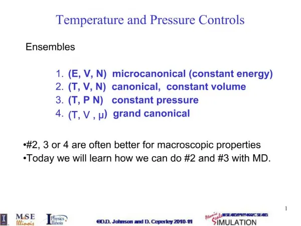
2. Introduction Molecular mechanics simulations usually sample the microcanonical (constant NVE) ensemble . What if we are interested in some other ensemble such as the canonical (constant NVT) or isothermal-isobaric (constant NPT)? What if we are studying a system that gets too hot? • Do a Monte Carlo calculation instead (canonical). • Modify the molecular mechanics.

3. Scaling/Constraining Methods Temperature is Simplest way to modify T: Temperature depends on velocities so correct the velocities every step to give desired temperature. Multiply by Where TWis the temperature that you want and T(t) is the temperature at time t.Simple, but crude and may inhibit equilibration.

4. More Sophisticated S/C “Encourage” the temperature in the direction you want by coupling it to a heat bath. Have • is the coupling parameter. If t=dtthe simpler form of scaling is recovered. Neither method samples the canonical ensemble.

5. More Sophisticated S/C Redefine equations of motion. Choose x such that To minimize the difference with Newtonian trajectories take This samples configurational part of canonical ensemble Note that it prevents changes in T but does not change it to a desired value

6. Example, S/C 10 atoms in a cell interacting via a Lennard-Jones Potential. Simulate using leap-frog algorithm (6.3.1)

7. Example, S/C Simulate for a while

8. Example, S/C Obtain these properties (10,000,000 steps between 65,0000 and 650,001 not shown).

9. Example, S/C Same system but with scaling to a temperature of about 300.

10. Example, S/C Same system but with scaling to a temperature of about 300.

11. Stochastic Collisions • Influence the system temperature by reassigning the velocity of a random particle (a “collision”). An element of Monte-Carlo. • The new velocity is from the Maxwell-Boltzmann distribution corresponding to the desired TW. • Between collisions sample a micro-canonical ensemble. It can be shown that overall the canonical ensemble is sampled. • Collision frequency is important. • Can also reassign some or all particle velocities.

12. Extended Systems • Have a thermal reservoir coupled to the system. • The reservoir has its own degree of freedom s and its own thermal inertia parameter Q. • Energy is conserved in the total system and the micro-canonical ensemble of the total system is sampled. • Two flavours: 1.Nosé type 2.Hoover type

13. Nosé Method The extra degree of freedom s which scales the real velocities and time step s has its own kinetic and potential energies (f is the number of degrees of freedom) It can be shown that the partition function of this system is

14. Nosé Method Also, for a given property A. Note that the total momentum and total angular momentum deviate from canonical by O(1/N). • Q measures coupling between reservoir and system.It should not be too high (slow flow) or too low (oscillations).

15. Example of Nosé Method System made up of 108 argon atoms. S. Nosé Mol. Phys. 52, 255 (1984).

16. Hoover Method Start with the Nosé method and redefine the time variable Thus eliminate s from equations of motion Samples a canonical ensemble and is more “gentle” than straight scaling.

17. An Aside: Ab Initio Molecular Dynamics (9.13.2-3) • In the Car-Parinello method (e.g. PAW) Molecular Dynamics is performed using forces derived from QM. • The nuclear and electronic degrees of freedom are relaxed simultaneously. • When doing dynamics the electronic part must not heat up too much. • Couple electronic and nuclear motions each to their own Nosé-Hoover thermostat.

18. Constant Pressure Pressure: Can maintain constant pressure by changing V, the volume of the box. Long range corrections are important. Here f represents the forces. Volume changes can be large: Gas in 20Å square box (volume 8000 Å3) has DVRMS=18,100 Å3. Use a bigger box.

19. Scaling/Constraining Can “encourage” the pressure in the direction desired by scaling box size by c Can redefine equations of motion Where c is pretty ugly. Get

20. Extended Systems • Have the system coupled to a ‘piston’ . • The piston has its own degree of freedom V and its own ‘mass’ Q. • Energy is conserved in the total system and the micro-canonical ensemble of the total system is sampled.

21. Anderson Method • Variables are scaled. • The ‘piston’ has its own kinetic and potential energies. • It can be shown that the time average of the trajectories derived equal the isoenthalpic-isobaric ensemble average to O(N-2).

22. Extended Systems • Again, the size of Q is important to avoid oscillations/slow exploration of phase space. • Changing the box shape is a special case of this. Not so useful for liquids but good for solids.

23. Stochastic Methods None yet developed.

24. Constant Temperature and Pressure The isobaric-isothermal (constant NPT) ensemble is often of interest. Achieved by combing methods already described, e.g. • Couple system with a pistonthen maintain temperature by the stochastic method including collisions with the piston. • Redefine equations of motion to constrain T and P Here (c+x) equals the previous definition of x and c is slightly less ugly than before. 3. Hoover’s formulation

25. What Method to Use? • Scaling is simple and easy and in the simplest case requires no parameters. Convergence may be a problem and do not sample cononical/isobaric/isobaric-isothermal ensemble. Good for equilibration. • Constraints a little more complicated but also require no parameters. Only keep T/P unchanged. • Stochastic approach is more stable than scaling but method is no longer deterministic. • Extended systems methods more complicated and require parameters. Nosé-Hoover thermostats enable the true canonical ensemble to be sampled.

26. Summary • One may want to constrain/choose temperature and/or pressure in a molecular dynamics simulation for a number of reasons. • The temperature can be fixed by a) scaling the velocities (partially or completely) or simply redefining the equations of motion so that T does not change, b) changing some or all of the velocities of the particles to a randomly selected member of the Maxwell- Boltzmann distribution of the desired T, c) couple the system to a heat bath • Analagous methods exist to chose/maintain a constant pressure. • Combinations of methods can be used to simulate a system at constant temperature and pressure.