Download
1 / 38
380 likes | 385 Views
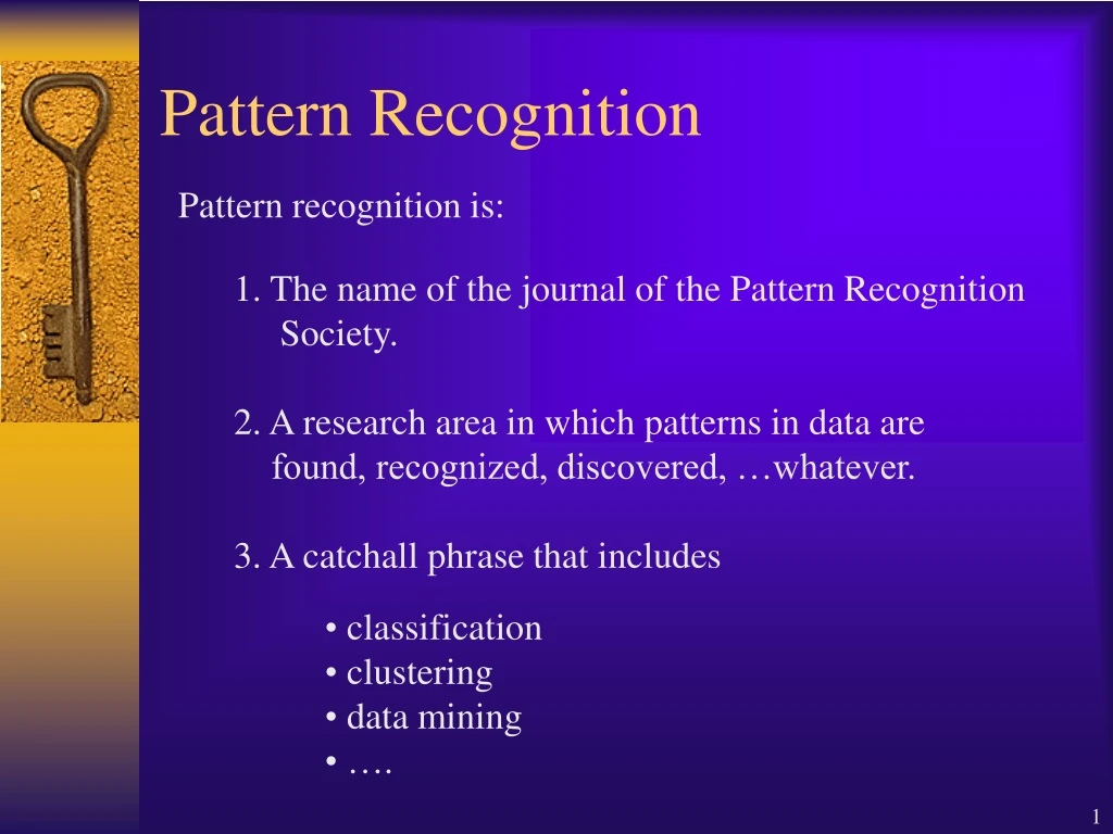
Pattern Recognition. Pattern recognition is:. 1. The name of the journal of the Pattern Recognition Society. 2. A research area in which patterns in data are found, recognized, discovered, …whatever. 3. A catchall phrase that includes. classification clustering data mining

E N D
Pattern Recognition Pattern recognition is: 1. The name of the journal of the Pattern Recognition Society. 2. A research area in which patterns in data are found, recognized, discovered, …whatever. 3. A catchall phrase that includes • classification • clustering • data mining • ….
Two Schools of Thought • Statistical Pattern Recognition • The data is reduced to vectors of numbers • and statistical techniques are used for • the tasks to be performed. • 2. Structural Pattern Recognition • The data is converted to a discrete structure • (such as a grammar or a graph) and the • techniques are related to computer science • subjects (such as parsing and graph matching).
In this course 1. How should objects to be classified be represented? 2. What algorithms can be used for recognition (or matching)? 3. How should learning (training) be done?
Classification in Statistical PR • A class is a set of objects having some important • properties in common • A feature extractor is a program that inputs the • data (image) and extracts features that can be • used in classification. • A classifier is a program that inputs the feature • vector and assigns it to one of a set of designated • classes or to the “reject” class. With what kinds of classes do you work?
Feature Vector Representation • X=[x1, x2, … , xn], each xj a real number • xj may be an object measurement • xj may be count of object parts • Example: object rep. [#holes, #strokes, moments, …]
Some Terminology • Classes: set of m known categories of objects (a) might have a known description for each (b) might have a set of samples for each • Reject Class: a generic class for objects not in any of the designated known classes • Classifier: Assigns object to a class based on features
Discriminant functions • Functions f(x, K) perform some computation on feature vector x • Knowledge K from training or programming is used • Final stage determines class
Classification using nearest class mean • Compute the Euclidean distance between feature vector X and the mean of each class. • Choose closest class, if close enough (reject otherwise)
Nearest mean might yield poor results with complex structure • Class 2 has two modes; where is its mean? • But if modes are detected, two subclass mean vectors can be used
Scaling coordinates by std dev We can compute a modified distance from feature vector x to class mean vector x by scaling by the spread or standard deviation of class c along each dimension i. scaled Euclidean distance from x to class mean x c i c
Nearest Neighbor Classification • Keep all the training samples in some efficient • look-up structure. • Find the nearest neighbor of the feature vector • to be classified and assign the class of the neighbor. • Can be extended to K nearest neighbors.
Receiver Operating Curve ROC • Plots correct detection rate versus false alarm rate • Generally, false alarms go up with attempts to detect higher percentages of known objects
Confusion matrix shows empirical performance Confusion may be unavoidable between some classes, for example, between 9’s and 4’s.
Bayesian decision-making • Classify into class w that is most likely based on • observations X. The following distributions are • needed. • Then we have:
Classifiers often used in CV • Decision Tree Classifiers • Artificial Neural Net Classifiers • Bayesian Classifiers and Bayesian Networks • (Graphical Models) • Support Vector Machines
Decision Trees #holes 0 2 1 moment of inertia #strokes #strokes t < t 1 0 best axis direction #strokes 0 1 4 2 0 90 60 - / 1 x w 0 A 8 B
Decision Tree Characteristics • Training • How do you construct one from training data? • Entropy-based Methods • 2. Strengths • Easy to Understand • 3. Weaknesses • Overtraining
Entropy-Based Automatic Decision Tree Construction Node 1 What feature should be used? Training Set S x1=(f11,f12,…f1m) x2=(f21,f22, f2m) . . xn=(fn1,f22, f2m) What values? Quinlan suggested information gain in his ID3 system and later the gain ratio, both based on entropy.
Entropy Given a set of training vectors S, if there are c classes, Entropy(S) = -pi log (pi) Where pi is the proportion of category i examples in S. c 2 i=1 If all examples belong to the same category, the entropy is 0 (no discrimination). The greater the discrimination power, the larger the entropy will be.
Information Gain The information gain of an attribute A is the expected reduction in entropy caused by partitioning on this attribute. |Sv| Gain(S,A) = Entropy(S) - ----- Entropy(Sv) |S| v Values(A) where Sv is the subset of S for which attribute A has value v. Choose the attribute A that gives the maximum information gain.
Information Gain (cont) Set S Attribute A v2 v1 vk Set S S={sS | value(A)=v1} repeat recursively Information gain has the disadvantage that it prefers attributes with large number of values that split the data into small, pure subsets.
Information Content The information content I(C;F) of the class variable C with possible values {c1, c2, … cm} with respect to the feature variable F with possible values {f1, f2, … , fd} is defined by: • P(C = ci) is the probability of class C having value ci. • P(F=fj) is the probability of feature F having value fj. • P(C=ci,F=fj) is the joint probability of class C = ci • and variable F = fj. • These are estimated from frequencies in the training data.
Example (from text) • X Y Z C • 1 1 I • 1 1 0 I • 0 0 1 II • 1 0 0 II How would you distinguish class I from class II?
Using Information Content • Start with the root of the decision tree and the whole • training set. • Compute I(C,F) for each feature F. • Choose the feature F with highest information • content for the root node. • Create branches for each value f of F. • On each branch, create a new node with reduced • training set and repeat recursively.
Artificial Neural Nets Artificial Neural Nets (ANNs) are networks of artificial neuron nodes, each of which computes a simple function. An ANN has an input layer, an output layer, and “hidden” layers of nodes. . . . . . . Outputs Inputs
Node Functions neuron i w(1,i) a1 a2 aj an output w(j,i) output = g ( aj * w(j,i) ) Function g is commonly a step function, sign function, or sigmoid function (see text).
Neural Net Learning That’s beyond the scope of this text; only simple feed-forward learning is covered. The most common method is called back propagation. We’ve been using a free package called NevProp. What do you use?
Support Vector Machines (SVM) • Support vector machines are learning algorithms • that try to find a hyperplane that separates • the differently classified data the most. • They are based on two key ideas: • Maximum margin hyperplanes • A kernel ‘trick’.
Maximal Margin Margin 1 0 1 1 0 1 0 Hyperplane 0 Find the hyperplane with maximal margin for all the points. This originates an optimization problem which has a unique solution (convex problem).
Non-separable data 0 1 0 0 0 0 1 1 1 0 1 0 1 0 1 1 0 0 0 1 0 What can be done if data cannot be separated with a hyperplane?
The kernel trick The SVM algorithm implicitly maps the original data to a feature space of possibly infinite dimension in which data (which is not separable in the original space) becomes separable in the feature space. Feature space Rn Original space Rk 1 1 1 0 0 0 1 0 0 1 0 0 Kernel trick 1 0 0 0 1 1
Our Current Application • Sal Ruiz is using support vector machines in his • work on 3D object recognition. • He is training classifiers on data representing deformations • of a 3D model of a class of objects. • The classifiers learn what kinds of surface patches • are related to key parts of the model • (ie. A snowman’s face)
EM for Classification • The EM algorithm was used as a clustering algorithm for image segmentation. • It can also be used as a classifier, by creating a Gaussian “model” for each class to be learned.