Download
1 / 55
550 likes | 556 Views
Multicast, Packet Scheduling, QoS. EE 122: Intro to Communication Networks Fall 2010 (MW 4-5:30 in 101 Barker) Scott Shenker TAs: Sameer Agarwal, Sara Alspaugh, Igor Ganichev, Prayag Narula http://inst.eecs.berkeley.edu/~ee122/

E N D
Multicast, Packet Scheduling, QoS EE 122: Intro to Communication Networks Fall 2010 (MW 4-5:30 in 101 Barker) Scott Shenker TAs: Sameer Agarwal, Sara Alspaugh, Igor Ganichev, Prayag Narula http://inst.eecs.berkeley.edu/~ee122/ Materials with thanks to Jennifer Rexford, Ion Stoica, Vern Paxsonand other colleagues at Princeton and UC Berkeley
Last Lecture: Routing Challenges • Resilience • Routing not reliable while reconverging after failures • Traffic Engineering • Routing algorithms don’t automatically spread load across available paths • Policy Oscillations • Policy autonomy makes oscillations possible • Current routing algorithms provide no way to resolve policy disputes
Meeting These Challenges • Augmenting LS with Failure-Carrying Packets • No packet drops during convergence • Requires change to packet header • Augmenting DV with Routing Along DAGs • Local adaptation prevents packet drops, spreads load • No need for header changes, applies to L2 and L3 • Augmenting PV with Policy Dispute Resolution • Only invoked when oscillation is in progress
Today’s Lecture • Last lecture preserved traditional service model • Unicast, best-effort delivery • Just made it more reliable • Today, we examine changes to the service model • Multicast: one-to-many delivery model • Quality of service: better than “best-effort” • Packet scheduling is a key component • But also useful in congestion control (later lecture) • Key architectural concept • Soft-state design
Motivating Example: Internet Radio • Live 8 concert • At peak, > 100,000 simultaneous online listeners • Could we do this with parallel unicast streams? • Bandwidth usage • If each stream was 1Mbps, concert requires > 100Gbps • Coordination • Hard to keep track of each listener as they come and go • Multicast addresses both problems….
Backbone ISP Unicast approach does not scale… Broadcast Center
Backbone ISP Instead build trees • Copy data at routers • At most one copy of a data packet per link Broadcast Center • LANs implement link layer multicast by broadcasting • Routers keep track of groups in real-time • Routers compute trees and forward packets along them
R1 joins G [G, data] [G, data] [G, data] R0 joins G [G, data] Rn joins G Multicast Service Model • Receivers join multicast group identified by a multicast address G • Sender(s) send data to address G • Network routes data to each of the receivers • Note: multicast is both a delivery and a rendezvous mechanism • Senders don’t know list of receivers • For many purposes, the latter is more important than the former R0 R1 S Net . . . Rn
Multicast and Layering • Multicast can be implemented at different layers • link layer • e.g. Ethernet multicast • network layer • e.g. IP multicast • application layer • e.g. End system multicast • Each layer has advantages and disadvantages • Link: easy to implement, limited scope • IP: global scope, efficient, but hard to deploy • Application: less efficient, easier to deploy [not covered]
Multicast Implementation Issues • How is join implemented? • How is send implemented? • How much state is kept and who keeps it?
Link Layer Multicast • Join group at multicast address G • NIC normally only listens for packets sent to unicast address A and broadcast address B • After being instructed to join group G, NIC also listens for packets sent to multicast address G • Send to group G • Packet is flooded on all LAN segments, like broadcast • Scalability: • State: Only host NICs keep state about who has joined • Bandwidth: Requires broadcast on all LAN segments • Limitation: just over single LAN
Network Layer (IP) Multicast • Performs inter-network multicast routing • Relies on link layer multicast for intra-network routing • Portion of IP address space reserved for multicast • 228 addresses for entire Internet • Open group membership • Anyone can join (sends IGMP message) • Privacy preserved at application layer (encryption) • Anyone can send to group • Even nonmembers • Flexible, but leads to problems
IP Multicast Routing • Intra-domain • Source Specific Tree: Distance Vector Multicast Routing Protocol (DVRMP) • Shared Tree: Core Based Tree (CBT) • Inter-domain [not covered today] • Protocol Independent Multicast • Single Source Multicast
Distance Vector Multicast Routing Protocol • Elegant extension to DV routing • Using reverse paths! • Use shortest path DV routes to determine if link is on the source-rooted spanning tree • Three steps in developing DVRMP • Reverse Path Flooding • Reverse Path Broadcasting • Truncated Reverse Path Broadcasting (pruning)
r Reverse Path Flooding (RPF) If incoming link is shortest path to source • Send on all links except incoming • Otherwise, drop Issues: • Some links (LANs) may receive multiple copies • Every link receives each multicast packet s:3 s:2 s:3 s:1 s:2 s
Other Problems • Flooding can cause a given packet to be sent multiple times over the same link • Solution: Reverse Path Broadcasting S x y a duplicate packet z b
forward only to child link Reverse Path Broadcasting (RPB) • Choose single parent for each link along reverse shortest path to source • Only parent forwards to child link • Identifying parent links • Distance • Lower address as tie-breaker S Parent of z on reverse path 5 6 x y a child link of x for S z b
Not Done Yet! • This is still a broadcast algorithm – the traffic goes everywhere • Need to “Prune” the tree when there are subtrees with no group members • Add the notion of “leaf” nodes in tree • They start the pruning process
Pruning Details • Prune (Source,Group) at leaf if no members • Send Non-Membership Report (NMR) up tree • If all children of router R send NMR, prune (S,G) • Propagate prune for (S,G) to parent R • On timeout: • Prune dropped • Flow is reinstated • Down stream routers re-prune • Note: a soft-state approach
Distance Vector Multicast Scaling • State requirements: • O(Sources Groups) active state • How to get better scaling? • Hierarchical Multicast • Core-based Trees
Core-Based Trees (CBT) • Pick a “rendevouz point” for the group (called core) • Build tree from all members to that core • Shared tree • More scalable: • Reduces routing table state from O(S x G) to O(G)
Use Shared Tree for Delivery • Group members: M1, M2, M3 • M1 sends data root M1 M2 M3 control (join) messages data
Barriers to Multicast • Hard to change IP • Multicast means changes to IP • Details of multicast were very hard to get right • Not always consistent with ISP economic model • Charging done at edge, but single packet from edge can explode into millions of packets within network • Troublesome security model • Anyone can send to a group • Denial-of-service attacks on known groups
5 Minute Break Questions Before We Proceed?
Announcements • Homework 3b coming soon!
Scheduling • Decide when and what packet to send on output link • Classifier partitions incoming traffic into flows • In some designs, each flow has their own FIFO queue flow 1 Classifier flow 2 Scheduler 1 2 flow n Buffer management
Packet Scheduling: FIFO • What if scheduler uses one first-in first-out queue? • Simple to implement • But everyone gets the same service • Example: two kinds of traffic • Video conferencing needs high bandwidth and low delay • E.g., 1 Mbps and 100 msec delay • E-mail transfers not very sensitive to delay • Cannot admit much e-mail traffic • Since it will interfere with the video conference traffic
Packet Scheduling: Strict Priority • Strict priority • Multiple levels of priority • Always transmit high-priority traffic, when present • .. and force the lower priority traffic to wait • Isolation for the high-priority traffic • Almost like it has a dedicated link • Except for the (small) delay for packet transmission • High-priority packet arrives during transmission of low-priority • Router completes sending the low-priority traffic first
50% red, 25% blue, 25% green Scheduling: Weighted Fairness • Limitations of strict priority • Lower priority queues may starve for long periods • … even if the high-priority traffic can afford to wait • Traffic still competes inside each priority queue • Weighted fair scheduling • Assign each queue a fraction of the link bandwidth • Rotate across the queues on a small time scale • Send extra traffic from one queue if others are idle
Max-Min Fairness • Given a set of bandwidth demands ri and a total bandwidth C, the max-min bandwidth allocations are: ai = min(f, ri) • where f is the unique value such that Sum(ai) = C • Property: • If you don’t get full demand, no one gets more than you • Max-min name comes from multi-good version
Computing Max-Min Fairness • Denote • C – link capacity • N – number of flows • ri – arrival rate • Max-min fair rate computation: • compute C/N (= the remaining fair share) • if there are flows i such that ri ≤ C/Nthen update C and Nandgo to 1 • ifnot, f = C/N; terminate
f = 4: min(8, 4) = 4 min(6, 4) = 4 min(2, 4) = 2 8 10 4 6 4 2 2 Example • C = 10; r1 = 8, r2 = 6, r3 = 2; N = 3 • C/3 = 3.33 • Can service all of r3 • Remove r3 from the accounting: C = C – r3 = 8; N = 2 • C/2 = 4 • Can’t service all of r1 or r2 • So hold them to the remaining fair share: f = 4
Fair Queuing (FQ) • Conceptually, computes when each bit in the queue should be transmitted to attain max-min fairness (a “fluid flow system” approach) • Then serve packets in the order of the transmission time of their last bits • Allocates bandwidth in a max-min fairly
Example Flow 1 (arrival traffic) 1 2 3 4 5 6 time Flow 2 (arrival traffic) 1 2 3 4 5 time Service in fluid flow system 1 2 3 4 5 6 1 2 3 4 5 time Packet system 1 2 1 3 2 3 4 4 5 5 6 time
Fair Queuing (FQ) • Provides isolation: • Misbehaving flow can’t impair others • Very important in congestion control (but not used) • Doesn’t “solve” congestion by itself: • Still need to deal with individual queues filling up • Generalized to WeightedFairQueuing (WFQ) • Can give preferences to classes of flows
OK, so now what? • So we know how to schedule packets • How does that improve the quality of service? • In particular, can we do better than “best-effort?
Differentiated Services (DiffServ) • Give some traffic better treatment than other • Application requirements: interactive vs. bulk transfer • Economic arrangements: first-class versus coach • What kind of better service could you give? • Fewer drops • Lower delay • Lower delay variation (jitter) • How to know which packets get better service? • Bits in packet header • Deals with traffic in aggregate • Very scalable
DS-2 DS-1 Egress Ingress Egress Ingress Edge router Core router Diffserv Architecture • Ingress routers - entrance to a DiffServ domain • Police or shape traffic (discussed later) • Set Differentiated Service Code Point (DSCP) in IP header • Core routers • Implement Per Hop Behavior (PHB) for each DSCP • Process packets based on DSCP
0 5 6 7 DS Field ECN 0 4 8 16 19 31 Version HLen TOS Length Identification Flags Fragment offset IP header TTL Protocol Header checksum Source address Destination address Data Differentiated Service (DS) Field • DS field encodes Per-Hop Behavior (PHB) • E.g., Expedited Forwarding (all packets receive minimal delay & loss) • E.g., Assured Forwarding (packets marked with low/high drop probabilities)
DiffServ Describes Relative Treatment • What if my application needs bounds on delay? • Integrated Services Architecture • Three steps necessary • Need to describe flow’s traffic • Need to reserve resources along path • Need to deny resource requests when overloaded
1: How to Characterize Flow’s Traffic • Option #1: Specify the maximum bit rate. • Maximum bit rate may be much higher average • Reserving for the worst case is wasteful • Option #2: Specify the average bit rate. • Average bit rate is not sufficient • Network will not be able to carry all of the packets • Reserving for average case leads to bad performance • Option #3: Specify the burstiness of the traffic • Specify both the average rate and the burst size • Allows the sender to transmit bursty traffic • … and the network to reserve the necessary resources
Maximum # of bits sent r bps bits slope r b·R/(R-r) b bits slope R ≤ R bps time b/(R-r) regulator Characterizing Burstiness: Token Bucket • Parameters • r – average rate, i.e., rate at which tokens fill the bucket • b – bucket depth (limits size of burst) • R – maximum link capacity or peak rate • A bit can be transmitted only when a token is available
(b) (a) 3Kb 2.2Kb T = 2ms : packet transmitted b = 3Kb – 1Kb + 2ms*100Kbps = 2.2Kb T = 0 : 1Kb packet arrives (c) (d) (e) 3Kb 2.4Kb 0.6Kb T = 4ms : 3Kb packet arrives T = 10ms : packet needs to wait until enough tokens are in the bucket T = 16ms : packet transmitted Traffic Enforcement: Example • r = 100 Kbps; b = 3 Kb; R = 500 Kbps
2: Reserving Resources End-to-End • Source sends a reservation message • E.g., “this flow needs 5 Mbps” • Each router along the path • Keeps track of the reserved resources • E.g., “the link has 6 Mbps left” • Checks if enough resources remain • E.g., “6 Mbps > 5 Mbps, so circuit can be accepted” • Creates state for flow and reserves resources • E.g., “now only 1 Mbps is available” • RSVP • Dominant reservation protocol
QoS Guarantees: Per-hop Reservation • End-host: specify • arrival rate characterized by token bucket with parameters (b,r,R) • the maximum tolerable delay D, no losses • Router: allocate bandwidth ra, buffer space Ba such that • no packet is dropped • no packet experiences a delay larger than D
QoS Guarantee: Per-Hop Reservations • End-host: specifies • Traffic token bucket with parameters (b,r,R) • Maximum tolerable delay D • Router: allocates bandwidth buffer space so that: • No packet is dropped • No packet experiences a delay larger than D • If it doesn’t have the spare capacity, it says no
Ensuring the Source Behaves • Guarantees depend on the source behaving • Extra traffic might overload one or more links • Leading to congestion, and resulting delay and loss • Solution: need to enforce the traffic specification • Solution #1: policing • Drop all data in excess of the traffic specification • Solution #2: shaping • Delay the data until it obeys the traffic specification • Solution #3: marking • Mark all data in excess of the traffic specification • … and give these packets lower priority in the network