Download
1 / 48
480 likes | 601 Views
ATHENS, GREECE NMDB TC. Part 2. Cosmic Rays entry from Heliosphere to Variable Magnetosphere. K. Kudela, IEP SAS Ko š ice, Slovakia, kkudela@kosice.upjs.sk http://space.saske.sk Athens, Greece, September 14, 2009. 1. Numerical solution of equation of particle motion .

E N D
ATHENS, GREECE NMDB TC Part 2. Cosmic Rays entry from Heliosphere to Variable Magnetosphere K. Kudela, IEP SAS Košice, Slovakia, kkudela@kosice.upjs.sk http://space.saske.sk Athens, Greece, September 14, 2009
1. Numerical solution of equation of particle motion. The differential equation describing trajectory of a particle (charge q, mass m) in the static magnetic field B(r) is given by d2r/dt2 = (q/m). dr/dt x B(1) This equation leads to system of 6 linear differential equations with unknown values (x, y, z, dx/dt, dy/dt, dz/dt) which is usually solved numerically (earlier e.g. Shea M.A. et al.,ERP 141, AFCRL-65-705, 1965; Flückiger, E.O., AFGL-TR-82-0320,1982 among others). We use the scheme of Runge-Kutta of 6th order or 4th order (Kaššovicová, J. and Kudela,K., preprint IEP SAS 1995; Bobík, P., PhD thesis, 2001).
Initial conditions: rigidity (velocity), charge, direction of access (zenith, azimuth angle) (x,y,z,vx,vy,vz), back tracing numerical integration of (1) in given B (x,y,z) from the point of observation in given direction with charge sign reversed. Time step (elementary straight line) is based on gyroperiod (according to local |B|;Dt=T/n; T is gyroperiod, n=100 usually). Conditions for smoothness of trajectory (angle between two subsequent elementary straight lines on trajectory < a, usually a = 0.001 rad) Conservation of initial module v (|v-vinitial|/|vinitial| < e, e = 10-4 usually) Conditions for finishing the trajectory tracing (N=max. number of steps, crossing earth, crossing magnetopause, N=50000 usually)
A B Examples of trajectory computations (projections to XYGSM plane). Position of Lomnický Štít, vertical access. A: allowed traj. B: R=3.25 GV forbidden C: R=2.25 GV quasitrapped C
2. Geomagnetic field models used for cosmic ray trajectory computations. Internal field: IGRF model The IAGA released the 10th Generation International Geomagnetic Reference Field — the latest version of a standard mathematical description of the Earth's main magnetic field. The coefficients for this degree and order 13 main field model were finalized by a task force of IAGA in Dec. 2004. (http://www.ngdc.noaa.gov/IAGA/vmod/igrf.html) The IGRF is a series of mathematical models of the Earth's main field and its annual rate of change (secular variation). In source-free regions at the Earth's surface and above, the main field, with sources internal to the Earth, is - grad (V), V - potential which can be represented by a truncated series expansion:
where r, θ, λ are geocentric coordinates (r is the distance from the centre of the Earth, θ is the co-latitude, i.e. 90° - latitude, and λ is the longitude), R is a reference radius (6371.2 km); and are the coefficients at time t and are the Schmidt semi-normalised associated Legendre functions of degree n and order m. The main field coefficients are functions of time and for the IGRF the change is assumed to be linear over five-year intervals. For the upcoming five-year epoch, the rate of change is given by predictive secular variation coefficients. We use the GEOPACK library: it consists of subsidiary FORTRAN subroutines for magnetospheric modeling studies, including the current (IGRF) and past (DGRF) internal field models, a group of routines for transformations between various coordinate systems, and a field line tracer. (http://modelweb.gsfc.nasa.gov/magnetos/data-based/geopack.html ) (http://modelweb.gsfc.nasa.gov/magnetos/data-based/Geopack_2005.html)
Structure of allowed and forbidden trajectories is different for different periods of time in the internal field approach. From paper (Storini, M. et al, Proc. ICRC, Rome, vol. 4, p. 1074-1077, 1995)
Vertical cut-off rigidities for many cosmic ray stations were computed for epochs 1955 – 1995 with 5 year step given by the IGRF models are in paper(M.A. Shea and D.F. Smart, Proc. ICRC, Hamburg, p. 4063-4066, 2001).
Cut-offs for non-vertical directions. For correct interpretation of responses of ground based cosmic ray measurement by detectors with omnidirectional chracteristics of acceptance (as NM are, part 3), the obliquely incident particle have to be taken into account too. One approach is e.g. in paper (J.M. Clem et al, J. Geophys. Res. 102, No A12, 26,919-26,926, 1997). An “apparent” cut-off is defined: Apparent cut-off is that rigidity which, if uniform over the whole sky, would yield the same neutron monitor counting rate as the real, angular dependent cutoff distribution. Cut-off sky-maps are computed. While this approach requires large computing time, In paper (J.W. Bieber et al, Proc. ICRC, Durban, 2, 389-392, 1997) simplification is checked: effective cutoffs are computed for 9 directions (vertical and ring 30 degrees off vertical with 8 directions by azimuth) and apparent cutoff is computed with corresponding statistical weights (vertical cutoff ½,other cutoffs with weight 1/16 each).
From paper (J.W. Bieber et al, Proc. ICRC, Durban, 2, 389-392, 1997)
External field (contributions of external current systems). We use A. Tsyganenko’89 model (Tsyganenko, N.A., Planet. Space Sci., vol. 37, No 1, pp. 1-20, 1989) Code at http://modelweb.gsfc.nasa.gov/magnetos/data-based/T89c.html Input parameters: IOPT – specifies the ground disturbance level: IOPT= 1, 2, 3, 4, 5, 6, 7 correspond to Kp= (0,0+),(1-,1,1+), (2-,2,2+), (3-,3,3+),(4-,4,4+), (5-,5,5+),(> =6-). Dipole tilt angle; x, y, z position in GSM. B.Tsyganenko’89 model with extension of Dst. Putting one parameter of model (A) as a parameter depending on Dst, an approach to geomagnetic transmission during the disturbances in October 1989 was proposed (Boberg, P.R. et al., 22, No 9, 1133-1136, 1995).
C. Tsyganenko’96 model (code at http://modelweb.gsfc.nasa.gov/magnetos/data-based/T96.html) Input parameters: solar wind pressure, Dst, By, Bz of IMF; dipole tilt angle; x, y, z position in GSM D. Tsyganenko 2001 model Input parameters: Dipole tilt angle; solar wind pressure; Dst; IMF By and Bz components; two IMF-related indices G1 and G2 taking into account the IMF and solar wind conditions during the preceding 1-hour interval (their definition is in paper available online from anonymous ftp://nssdcftp.gsfc.nasa.gov/models/magnetospheric/tsyganenko/2001paper/)
E. Tsyganenko 2004 model Model of the external (i.e. without earth’s contribution) part of the magnetospheric field, calibrated by solar wind pressure; Dst; By of IMF; Bz IMF and indices W1 – W6 calculated as time integrals from beginning of a storm (Bz, n, v; described in N. A. Tsyganenko and M. I. Sitnov, Modeling the dynamics of the inner magnetosphere during strong geomagnetic storms, JGR v. 110, 2005, J. Geophys. Res., vol. 110, A03208, doi:10.129/2004JA010798, 2005); dipole tilt angle; x,y,z GSM position
3. Effects of magnetosheric disturbances on cosmic rays. Diurnal variation of the cut-off rigidity. While IGRF is not sensitive to local time of measurements, the external field models assume the local time asymmetry of magnetosphere. For a middle latitude station Lomnický Štít the structure of allowed (black) and forbidden (white) trajectories is depending on local time and on level of geomagnetic disturbance (Left for IOPT=1, right IOPT=6, 21.3.1990), vertical directions. Ts89 model (A) is used (P. Bobík, PhD thesis, 2001).
Variation of RE (effective vertical cut-off rigidity in GV)for position of Lomnický Štít (left panel) and LARC (right panel) with local time of measurements according to Ts89 model (A). Computations are done for January 21, 1986. At high latitude stations the diurnal variation of cut-off rigidity is not important since the cut-off rigidity is below the atmospheric one (about 400 MeV kinetic energy p).
Average transmissivity. Computing trajectories with small step in rigidity (0.0001 GV) gives the probability that particlehaving rigidity e.g. in the interval (R,R+0.01) GV can access the site. TF (transmissivity function) is used for such probability. TF computed for Lomnický Štít, 24 hour averaged for different levels of geomagnetic activity (Ts89 model (A) used). Kudela,K. and Usoskin,I.G, Czech. J. Phys, 54, 239-254, 2004.
Transmissivity function for Lomnický Štít averaged over long time period with different Kp indices and over diurnal change of the cut-off rigidities. TF can be used for analysis of long term variations of cosmic rays observed at a particular station.
Asymptotic directions for middle latitude station at low rigidity interval for different models of the magnetic field. Upper panels are for Ts’89 model (A); lower panels are for the model with Dst extension (B). The different asymptotics are seen also for local noon and midnight.
Change of asymptotic directions at a high latitude station (Inuvik) in dependence on geomagnetic activity level. Rigidities 0.3 - 20 GV are displayed (P. Bobík, PhD thesis, 2001)
Changes of asymptotic directions due to geomagnetic activity. Asymptotic directions for particles vertically accessing Lomnický Štít for low and high geomagnetic activity level. Ts89 model (A) is used. Rigidities 4.1-4.5 GV are marked by crosses, interval 4.5-20 GV by circles. (Bobík, P., PhD thesis, 2001)
Time profile of cut-off depression, asymptotic directions and transmissivity function are different for different models.
Example. November 20-22, 2003. Isolated Dst depression. Improvement of magnetospheric transmissivity is clearly seen at NMs with high cut-off rigidities.
Similarly to that case the increase at Tibet neutron monitor (nominal vertical cut-off ~14.1 GV) was observed during a couple of geomagnetic storms (Miyasaka H. et al, Proc. ICRC Tsukuba, 6, 3609-3612, 2003).
For interval 2 data for using Ts04 model are available. Differences in transmissivity of CR in different models can be tested. Tsyganenko 04 model uses “prehistory” of geomagnetic storm. Input parameters W1(inner tail current), W2(outer tail current), W3(symmetrical ring current), W4 (partial ring current), W5 (FAC-region 1), W6 (FAC-region 2). Constructed from the time profiles of Np, Vp, IMF Bz by Tsyganenko and Sitnov, 2005 formula (7)modified for one – hour data. Computations by Bučík.
Differences of Ts89, Ts89+Dst, Ts04: 1. Transmissivity function: Ts89 Ts89+Dst Ts04 TF (for vertical direction) for Lomnický Štít before the onset of the storm (Nov. 20, 2003, 02 UT, black) and during the Dst minimum (19 UT, red) for three models. (Kudela, Bučík and Bobík, 2008).
2. Asymptotics. Asymptotic directions for Lomnický Štít before the disturbance (upper panels, Nov. 20, 2003, 02 UT) and at minimum Dst (lower panels, 19 UT) for Ts89+Dst (left) and Ts04 (right).
3. Timing of minimum cut-off rigidity. Rome neutron monitor. Increase in CR is matching better the cut-off decrease for Ts04 model than that for Ts89 + Dst.
Different models give different asymptotic directions during high level of geomagnetic activity (computations by R. Bučík, 2005). Model B, 20.11.03, 19 UT Model E, 20.11.03, 19 UT LomnickýŠtít Model B, 8.11.04, 06 UT Model E, 8.11.04, 06 UT Mexico
How to check validity of geomagnetic field models by CR during geomagnetic storms? Timing of maximum CR increase vs min. predicted cut-off at many stations (?) Very simplified: simultaneous change of CR anisotropy in interplanetary space (CME passing Earth’s orbit) Spaceship Earth (Bieber J.W., P. Evenson, ICRC, 1995), ring of NM at high latitudes – anisotropy at low energies (not strongly affected by magnetospheric disturbance – asymptotic directions in narrow interval of longitudes, close to ecliptic, changes below atmospheric cutoff) – ref. for IP anisotropy at LE ? Network of muon directional telescopes (Munakata K. et al., Adv. Space Res., 2005) studies anisotropy at energies above NM (~50 GeV), not strongly affected by changes in magnetosphere – ref. for IP anisotropy at HE ?
4. Transmissivity computed for low earth orbits. There are differences of transmissivity function at low earth orbit for different geomagnetic field models and for different levels of geomagnetic activity. Using tables of asymptotic directions and vertical cut-off rigidities computed in IGRF field (Shea, M.A., D.F. Smart, Environ. Res. Pap. 503, AFCRL-TR-75-0185, pp165, Bedford, Mass., 1975), the vertical cut-offs for altitudes >20 km were approximated by (Heinrich,W. and Spill,A., J. Geophys. Res., 84, A8, 4401-4404, 1979) by using the approximation Rc(1)/Rc(2)=L2(1)/L2(2) where Rc(1) and Rc(2) are vertical cut-off values on the same radius vector from the center of earth and L is McIlwain parameter of the magnetic field shell.
Transmissivity function (TF) for defined direction: Trajectory computations with dR step (dR < DR). TF(R,DR) is probability that particle of rigidity (R,R+DR) can access the given point in the model field. Introduced for description of fine structure of penumbra (e.g. Bobík, P. et al., ICRC 2001; Kudela and Usoskin, Czech. J. Phys., 2004) Earlier: Cutoff probability (Heinrich and Spill, J. Geophys. Res., 1979), Geomagnetic transmission in disturbed magnetosphere (Boberg et al, Geophys. Res. Lett., 1995)
TF=1 During the strong disturbances the penumbra at low altitudes has rather complicated structure (Kudela, K. and I.G. Usoskin, Czech. J. Phys,54, 239-254, 2004). There appear windows for relatively low rigidities. TF 1.07-1.08 GV 0.86-0.87 GV (TF=1)
Application of TF Expected by TF measurements In penumbra the observed energy spectra (AMS) showed the excess above those expected by primary cosmic ray (CREME96 model) and by TF - estimate of contribution of secondary CR (mainly re-entrant albedo protons), Bobík, P. et al., J. Geophys. Res. 2006. For one cut-off interval.
Plot of the differential energy spectrum of PAMELA at different values of geomagnetic cutoff G. It ispossible to see the primary spectrum at high rigidities and the reentrant albedo (secondary) flux at low rigidities. From De Simone et al, ICRC 2009, PAMELA collaboration.
Charged particles, low orbits. Example 1. Oct. 28-29, 2003. CORONAS-F. Oct. 28, 2003 before (left panel) and during the storm (right panel): proton flux profiles J (# /cm2.s.sr). Background, full line (26.10.) and dashed one (28.10.) almost identical. Right panel – comparison of profiles after arrival of high energy protons (full line) with background (dashed) indicates clear excess at L > 2. Checked 4 x per orbit. The increase (decline from background) started at 1120 UT on 28.10. and was observed from L=1.75 to L=3.5 (Kuznetsov et al, 2007) p>90 MeV, e > 75 MeV
GOES flux of protons E > 700 MeV (cm2.s.sr) -1 Fluxes of protons E > 90 MeV observed ad various L crossings by SONG/CORONAS-F. Linear scale, relative units vs background (DN/N %) Assuming spectral shape J (>E) = Jo . E-g Values are fitted for all crossings. Circles and white romboids – morning sector (north, south) Dots and black romboids – evening sector (north,south) Lines – 3 h averages g Jo
For trajectory (at L=1.75, 2.0, 2.25, 2.75, 3.0 and 3.5) the vertical cutoff rigidities were computed at each point according to Ts’89 model (Tsyganenko, PSS, 1989), more details in paper by Kuznetsov et al, 2006, 2007). Using power-law energy spectra, values Jo andg wereobtained. One of the energy spectra obtained from SONG data: at 1142-1146 UT evening sector (black squares) and at 1204-1209 UT morning sector (circles) Comparison with NM data (line > 400 MeV) according to Vashenyuk et al (Izv. RAN, 2005) and Miroshnichenko et al. (JGR, 2005) J (m2.sr.s.GeV) -1 Increase during event 29.10. – more complicated – strong magnetic activity For event November 2 fit g ~3.5 (around 2128 UT) E (GeV)
Example 2. December 13, 2006, PAMELA. Proton differential energy spectra (flux vs kinetic energy) in different time intervals during the event of the13th December 2006. From De Simone et al, ICRC, 2009.
Time profiles of p flux for wide energy range (upper panel); evolution of the spectra (bottom) based on PAMELA data (From De Simone et al, ICRC, 2009)
Three-hour averaged cutoff rigidity contours for Kp = 2 for hours 00 UT (left side) and 12 UT (right side). Top panel: the northern hemisphere.Bottom panel, the southern hemisphere. From Smart et al., 2006; Smart and Shea, 2009.
Three-hour averaged cutoff rigidity contours for Kp = 5 for hours 03 UT (left side) and 15 UT (right side). Top panel: the northern hemisphere.Bottom panel, the southern hemisphere. From Smart et al., 2006; Smart and Shea, 2009.
Boundary of penetration depends on geomagnetic activity. Dependences of the SEP penetration boundaries on(a) Dst and (b)Kpin the evening and night MLT sectors:invariant latitudes of the penetration boundaries for protons(squares) 1–5 and (triangles) 50–90 MeVand linear regressionfor (1–5)-MeV and(50–90)-MeV protons (solid and dashed lines, respectively) CORONAS-F. From Myagkova et al, 2009. Interval 2001-2005.
5. Long term variability of CR access to vicinity of Earth. Parts 2 and 3 are based on models of the geomagnetic field valid for the recent period. However, geomagnetic field was changing on long time scales. There are positions on the earth where the geomagnetic cut-offs are changing over past century more dramatically than in another positions. The vertical cut-off can be approximated as a function of L, McIlwain’s parameter (e.g. Shea, M. A. et al, Phys. Earth and Planet. Interiors, 48, 200-205,1987). While around 1950 positions of LŠ and LARC (in opposite hemispheres) had almost the same value L, by the end of last century L at LARC was significantly higher (lower cut-off) than at LŠ (Kudela,K. and M. Storini, Proc. ICRC, Hamburg, 9,4106-4109, 2001) L LARC position LŠ
Changes of geomagnetic cut-offs in the past: available models of geomagnetic field are used (e.g. Kudela, K., Bobík, P., Solar Phys., 224, N 1-2, 423 – 431, 2004).Different positions on earth had different cut-off rigidity time changes.
Lines of constant vertical cut–offs during the interval of years 0 to 2000. Computations done from available magnetic field models.
The “global transmission function”: the fraction of the Earth’s surface at which the vertical access of cosmic rays for R > Rcis allowed for different epochs. Earth was in the past exposed to cosmic rays in changing manners.