Download
1 / 37
370 likes | 526 Views
Physically-Based Visual Simulation on Graphics Hardware. Mark J. Harris Greg Coombe Thorsten Scheuermann Anselmo Lastra. More, Better, Faster. Goal: Flexible, real-time visual simulation of diverse dynamic systems Further increase visual realism of interactive 3D applications

E N D
Physically-Based Visual Simulation on Graphics Hardware Mark J. Harris Greg Coombe Thorsten Scheuermann Anselmo Lastra
More, Better, Faster • Goal: • Flexible, real-time visual simulation of diverse dynamic systems • Further increase visual realism of interactive 3D applications • Fluids, gases, fire, etc. • Beyond canned texture animations
Visual Simulation? • Goal is visual realism • Ad hoc simulation methods can provide good visual results w/ less computation • But not necessarily high numerical accuracy • If the user is convinced, numbers aren’t so important
Coupled Map Lattice • Mapping: • Continuous state lattice nodes • Coupling: • Nodes interact with each other to produce new state according to specified rules
Coupled Map Lattice • CML introduced by Kaneko (1980s) • Used CML to study spatio-temporal chaos • Others adapted CML to physical simulation: • Boiling [Yanagita 1992] • Convection [Yanagita 1993] • Clouds [Yanagita 1997; Miyazaki 2001] • Chemical reaction-diffusion [Kapral ‘93] • Saltation (sand ripples / dunes) [ Nishimori ‘93] • And more
CML vs. CA • CML extends cellular automata (CA)
CML vs. CA • Continuous state is more useful • Discrete: physical quantities difficult • Must filter over many nodes to get “real” values • Continuous: physical quantities easy • Real physical values at each node • Temperature, velocity, concentration, etc.
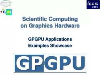
Graphics Hardware • Why use it? • Speed: up to 25x speedup in our sims • GPU perf. grows faster than CPU perf. • Cheap: GeForce 4 Ti 4200 < $140 • Load balancing in complex applications • Why not use it? • Low precision computation (not anymore!) • Difficult to program (not for long!)
CML Operations • Implement operations as building blocks for use in multiple simulations • Diffusion • Buoyancy (2 types) • Latent Heat • Advection • Viscosity / Pressure • Gray-Scott Chemical Reaction • Boundary Conditions • User interaction (drawing) • Transfer function (color gradient)
Results • Implemented multiple simulations • Boiling (2D and 3D) • Rayleigh-Bénard Convection (2D) • Reaction-diffusion (2D and 3D)
Boiling • [Yanagita 1992] • State = Temperature • Three operations: • Diffusion, buoyancy, latent heat • 7 passes in 2D, 9 per 3D slice
Rayleigh-Bénard Convection • [Yanagita & Kaneko 1993] • State = temp. (scalar) + velocity (vector) • Three operations (10 passes): • Diffusion, advection, and viscosity / pressure
Reaction-Diffusion • Gray-Scott reaction-diffusion model [Pearson 1993] • State = two scalar chemical concentrations • Simple: just diffusion and reaction ops • 2 passes in 2D, 3 per 3D slice
Hardware Limitations • Precision, precision, precision! • 8 or 9 bits is far from enough • Diffusion is very susceptible to precision problems • All of our simulations use it! • High dynamic range simulations are very susceptible • Convection, reaction-diffusion • Not boiling – relatively small range of values
Hardware Limitations • 3D texturing • It’s fast … unless you are doing dynamic texturing • Copy to slice of 3D texture is slow • We use a stack of 2D slices to represent 3D volume • Not all 2D texture shaders have 3D analogs • Fixed with general purpose fragment programs (NV30, ATI R300)
Future Work • Explore simulation techniques / issues on graphics hardware • Other PDE solution techniques • More complex simulations • Use of HLSL, next-gen hardware • High dynamic range simulations • Applications: • Interactive environments, games • Scientific Computation • Dynamic painting / modeling applications • Dynamic procedural texture synthesis • Dynamic procedural model synthesis • …
Conclusion GPUs are a capable, efficient, and flexible platform for physically-based visual simulation
Acknowledgements • NVIDIA Developer Relations • HWW Paper Reviewers • Sponsors: • NVIDIA Corporation • US National Institutes of Health • US Office of Naval Research • US Department of Energy ASCI program • US National Science Foundation
For More Information • http://www.cs.unc.edu/~harrism/cml • Email harrism@cs.unc.edu
CML Philosophy • Bottom-up approach. • Don’t directly simulate macroscopic behavior: • Perform simple, local, “microscopic” lattice operations.
CML Philosophy • Macroscopic behavior is aggregate of simple operations. • e.g. Boiling simulation: • 3 operations: diffusion, thermal buoyancy, latent heat.
CML Operations • Typically consist of four components: • Neighbor sampling • Computation on Neighbors • New state computation • State update
Neighbor Sampling • Set a 1:1 mapping from pixels to texels: • Set view port resolution to texture resolution. • Use orthographic projection. • To sample an immediate neighbor of each texel: • Draw a single quad filling the view port. • Set texture coordinates at corners to {(0,0), (0,1), (1,1), (1,0)} plus the offset to the neighbor. • E.G. Offset to right is (w, 0), whereis view space texel width.
Neighbor Sampling • Neighbor sampling is easy with vertex programs. • Store table of offsets in vertex program memory. • At run time, pass table index that represents the type of offset needed. • Render a quad (with only a single set of base texcoords). • Use vertex program to add offsets and generate texcoords for all texture units.
Computation on Neighbors • Use texture table lookups to compute arbitrary functions of sampled values. • Dependent texturing using texture shaders.
New State Computation • Combine sampled values and computations to compute new state. • Implemented on GeForce 3 using register combiners. • Arithmetic: add, subtract, multiply, scale, bias and dot product. • 8 cascaded register combiners + 1 “final” combiner. • 9-bit signed arithmetic internally. • 8-bit unsigned on output (can clamp or scale and bias).
State Update • Store the newly computed state to texture. • We use glCopyTexSubImage2D() • Fast copy from frame buffer to texture memory. • Render to texture OpenGL extension • Will reduce cost, but still in development. • Already available in Direct3D.
Common Operations • Laplacian: • Discrete form: • Diffusion: cd is the diffusion coefficient
Common Operations • Directional forces • Buoyancy (used in convection simulation): • Thermal buoyancy with phase change: • Uses dependent texture to compute tanh • Tcis the boiling point
Boiling Simulation Performance 25x speedup
Interactive Framework • CMLlab • Framework for building and testing CML simulations
Real Applications • Fast simulation integrated with 3D environments • Virtual environment in HMD w/ head tracking • WildMagic Game Engine [Eberly 2001]
Graphics Hardware Performance 9 10 One-pixel polygons (~10M polygons @ 30Hz) GeForce 3 & Radeon 8 10 Slope ~2.4x/year UNC/HP PixelFlow SGI R-Monster (Moore's Law ~ 1.7x/year) SGI Peak 7 IR 10 Nvidia TNT E&S Perf. Division Pxpl6 3DLabs SGI Cobalt Harmony UNC Pxpl5 Glint ('s/sec) Accel/VSIS SGI SkyWriter Voodoo 6 10 Megatek SGI VGX SGI E&S Freedom RE1 PC Graphics HP TVRX SGI RE2 HP VRX Flat shading Division VPX E&S 5 10 Textures Stellar GS1000 F300 UNC Pxpl4 SGI GT Antialiasing Gouraud shading HP CRX SGI Iris 4 10 86 88 90 92 94 96 98 00 Year Graph courtesy of Professor John Poulton