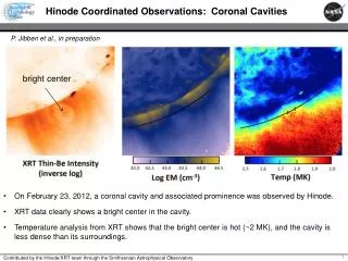
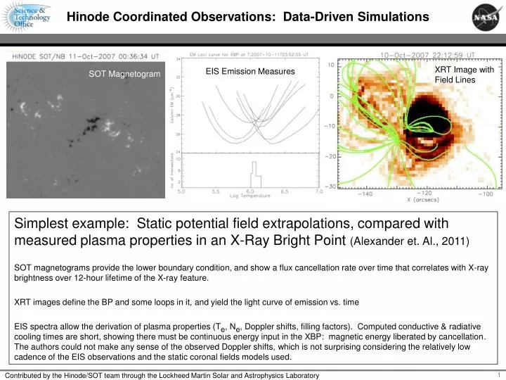
Hinode Coordinated Observations: Data-Driven Simulations

1. Hinode Coordinated Observations: Data-Driven Simulations XRT Image with Field Lines EIS Emission Measures SOT Magnetogram Simplest example: Static potential field extrapolations, compared with measured plasma properties in an X-Ray Bright Point (Alexander et. Al., 2011) SOT magnetograms provide the lower boundary condition, and showa flux cancellation rate over time that correlates with X-ray brightness over 12-hour lifetime of the X-ray feature. XRT images define the BP and some loops in it, and yield the light curve of emission vs. time EIS spectra allow the derivation of plasma properties (Te, Ne, Doppler shifts, filling factors). Computed conductive & radiative cooling times are short, showing there must be continuous energy input in the XBP: magnetic energy liberated by cancellation. The authors could not make any sense of the observed Doppler shifts, which is not surprising considering the relatively low cadence of the EIS observations and the static coronal fields models used. Contributed by the Hinode/SOT team through the Lockheed Martin Solar and Astrophysics Laboratory

2. Hinode Coordinated Observations: Data-Driven Simulations 3-D MHD Simulation of the corona above a quiescent Active Region (Bourdin et al., 2013) SOT magnetogramsand horizontal flows are the lower boundary conditions; an additional, artificial fine-scale flow is added to see if the resulting field-line braiding can cause the coronal heating. Loops are identified both in XRT and STEREO Fe XV images, and their 3-D geometry is reproduced fairly well with the simulation. The authors conclude that field-line braiding can heat the corona in this region but can’t exclude other possibilities. A spectral synthesis code computes line profiles of coronal lines observed by EIS. The main long loops in the AR “core” and the short loops in the lower left are synthesized. Both observed and model Doppler shifts show rising loop tops in the AR core and draining down both legs. Contributed by the Hinode/SOT team through the Lockheed Martin Solar and Astrophysics Laboratory

3. Hinode Coordinated Observations: Data-Driven Simulations IRIS 3-D Magneto-frictional model of an AR with Recurring Jets, using Bz and Jzon the photosphere (Cheung et al., 2014) Four similar jets were observed by SOT, EIS, XRT, SDO & IRIS. IRIS & EIS raster scans show highly asymmetric line profiles, with tails extending far beyond +/- 100 km/s. Helical (out-of-plane) motion is observed directly from Doppler shifts and indirectly from proper motions in all the jets Vector magnetograms from SP and HMI and the simple data-driven model point to an energy build-up mechanism previously suggested by Pariat et al. (2010): field lines twisted by persistent currents and rotation and rotation of an opposite-polarity pore. Two episodes of abrupt changes in the simulation with signs of untwisting fields are similar in appearance to the observed jets. Top View Side Views X Y Simulation Movie Orange ~ ∫los<j2>dl, where <j2> is fieldline-averaged j2 Green Positive polarity Br, Blue Negative polarity Br Contributed by the Hinode/SOT team through the Lockheed Martin Solar and Astrophysics Laboratory