PaRoNaMa WORKING GROUP

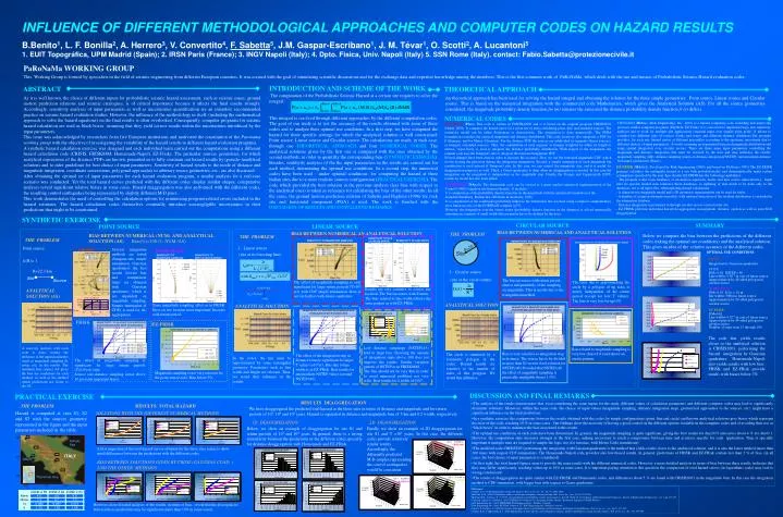
1. R=22.3 km Site 2r Source fR(r) = D2min –(L/2)2 L=103.9 km with Dmin< r < L r2-D2min Dmin=22.4 km Site SENSITIVITY TO LINE WIDTH INFLUENCE OF DIFFERENT METHODOLOGICAL APPROACHES AND COMPUTER CODES ON HAZARD RESULTS B.Benito1, L. F. Bonilla2, A. Herrero3, V. Convertito4, F. Sabetta5, J.M. Gaspar-Escribano1, J. M. Tévar1, O. Scotti2, A. Lucantoni51. EUIT Topográfica, UPM Madrid (Spain); 2. IRSN Paris (France); 3. INGV Napoli (Italy); 4. Dpto. Fisica, Univ. Napoli (Italy) 5. SSN Rome (Italy). contact: Fabio.Sabetta@protezionecivile.it PaRoNaMa WORKING GROUP This Working Group is formed by specialists in the field of seismic engineering from different European countries. It was created with the goal of stimulating scientific discussions and for the exchange data and expertise knowledge among the members. This is the first common work of PaRoNaMa, which deals with the use and misuse of Probabilistic Seismic Hazard evaluation codes. INTRODUCTION AND SCHEME OF THE WORK ABSTRACT THEORETICAL APPROACH The computation of the Probabilistic Seismic Hazard at a certain site requires to solve the integral: This integral is resolved through different approaches by the different computation codes. The goal of our study is to test the accuracy of the results obtained with some of these codes and to analyze their optimal use conditions. In a first step, we have computed the hazard for three specific settings for which the analytical solution is well constrained: Point source, Linear source and Circular source. The calculations are made, in each case, through one THEORETICAL APPROACH and four NUMERICAL CODES. The analytical solutions given by the first one is compared with the ones obtained by the second methods, in order to quantifiy the corresponding bias (SYNTHETIC EXERCISE). Besides, sentitiyity analyses of the the input parameters in the results are carried out for each method, determining the optimal use conditions. In a second step, the numerical codes have been used – under optimal conditions- for computing the hazard at three Italian sites due to a more realistic sources configuration (PRACTICAL EXERCISE). The code which provided the best solution in the previous analysis (less bias with respect to the analytical ones) is taken as reference for calculating the bias of the other results. In all the cases, the ground motion prediction relation of Sabetta and Pugliese (1996) for rock site and horizontal component (PGA) is used. The work is finished with the DISCUSSION OF RESULTS AND CONCLUDING REMARKS. As it is well known, the choice of different inputs for probabilistic seismic hazard assessment, such as seismic zones, ground motion prediction relations and seismic catalogues, is of critical importance because it affects the final results strongly. Accordingly, sensitivity analyses of input parameters as well as uncertainties quantification are an extended, recommended practice on seismic hazard evaluation studies. However, the influence of the methodology in itself, (including the mathematical approach to solve the hazard equations) on the final results is often overlooked. Consequently, computer programs for seismic hazard calculation are used as black boxes, assuming that they yield correct results within the uncertainties introduced by the input parameters. This issue was acknowledged by researchers from five European institutions and motivated the constitution of the Paronama working group with the objective of investigating the variability of the hazard results to different hazard evaluation programs. A synthetic hazard calculation exercise was designed and each individual team carried out the computations using a different hazard calculation code (CRISIS, FRISK88M, Homemade-Napoli, EZ-Frisk). The particular sources geometries, for which analytical expressions of the distance PDFs are known, permitted us to fully constrain our hazard results by (pseudo-)analytical solutions and to infer guidelines for best choice of input parameters. Sensitivity of hazard results to the mode of distance and magnitude integration, coordinate conversions, polygonal approaches to arbitrary source geometries, etc., are also discussed. After obtaining the optimal set of input parameters for each hazard evaluation program, a similar analysis for a real-case scenario was conducted. Yet the total hazard curves predicted with the different codes display similar shapes, comparative analyses reveal significant relative biases in some cases. Hazard deaggregation was also performed with the different codes, the resulting control earthquakes being represented by slightly different M-D pairs. This work demonstrates the need of controlling the calculation options for minimizing program-related errors included in the hazard estimates. The hazard calculation codes themselves eventually introduce non-negligible uncertainties in their predictions that ought to be constrained. An theoretical approach has been used for solving the hazard integral and obtaining the solution for the three simple geometries: Point source, Linear source and Circular source. This is based on the numerical integration with the commercial code Mathematica, which gives the Analytical Solution (AS). For all the source geometries considered, the magnitude probability density function fm (m) remains the same and the distance probability density function fr (r) differs. NUMERICAL CODES FRISK88M(ROma) (Risk Engineering, Inc., 2001) is a hazard computing code extending and improving previous similar computer programs (EQ-Risk, EZ-Frisk). It is conceived to implement logic tree sensitivity analyses and to work for multiple site applications (regional maps over regular point grids). It allows to consider two different type of sources (faults and areas) and different distance definitions.The program provides, for each site, hazard curves at different percentiles according to the epistemic uncertainty due to different choices of input parameters . It works assuming an exponential truncated magnitude distribution and using spatial integration over circular sectors. There are three main input parameters controlling the magnitude and distance integration that must be selected by the user and may influence the results: magnitude sampling (dM), distance sampling (range-of-distance-integration/NSTEP), and maximum distance for hazard calculations (Rmax). CRISIS2003(PAris) This code is written in FORTRAN90 and it is based on the original program CRISIS2001 (Ordaz, 2001). It computes the hazard curve for a given site or sites considering point, line, and extended sources. The seismicity model can be either Poissonian or characteristic. The integration is done numerically. The PSHA formulation considers the classical magnitude and distance distribution. This code, however, also integrates a PDF for β (Gamma), and for Mmax (Gaussian). For the distance PDF, the sources are subdivided in segments (linear sources), or triangles (extended sources). Thus, the contribution of each segment or triangle weighted by either its length or surface, respectively, is used to integrate the distance probability distribution. With respect to the magnitude, the original code uses the Simpson's rule to integrate the truncated magnitude PDF. Several changes have been done in order to increase the accuracy. First, we use the truncated magnitude CDF, which avoids loosing the precision during the integration summation. Second, a simple summation of each magnitude bin contribution is used instead of Simpson's rule. In this case, we can control the magnitude step, and it is useful for deaggregation purposes as well. Third, a Gauss quadrature is done when no deaggregation is needed. In this case the integration on the magnitude is independent on the magnitude step. Finally, the Youngs and Coppersmith (1985) seismicity model has also been added. • EZ-FRISK (MAdrid). Developed by Risk Engineering (2004) and based on McGuire (1995) The EZ-FRISK program calculates the earthquake hazard at a site both probabilistically and deterministically under certain assumptions specified by the user. Specifically, EZ-FRISK has the following capabilities: • - The program works from databases of attenuation equations, faults, and area source characteristics. Input files for specific hazard runs reference these databases, so updating of data needs to be done only to the databases, not to all input files, when updating hazard calculations. • A characteristic magnitude model and a 3D geometric representation can be used for faults. • A number of common attenuation models, with optional truncation of the residual distribution, is included in the attenuation database. • Distance integration is performed in through circular sectors centred at the site. • EZ-FRISK performs individual hazard de-aggregation in magnitude, distance, epsilon as well as joint M-D deaggregation HOMEMADE(NApoli). The homemade code can be viewed as a quasi explicit numerical implementation of the Cornell (1968)'s equation (no fineness herein). It includes : 1/ a computation of the probability density function on the magnitude with the analytical formulation of the bounded Gutenberg Richter law (McGuire & Arabasaz, 1990) 2/ a computation of the conditional probability linked to the attenuation law resolved using a implicit complementary error function (erfc) of the FORTRAN compiler (g77). However, the integration over the source zones (probability density function on the distance) is solved numerically summing arc segment of small width (this parameter has to be defined by the user). SYNTHETIC EXERCISE CIRCULAR SOURCE SUMMARY POINT SOURCE LINEAR SOURCE BIAS BETWEEN NUMERICAL AND ANALYTICAL SOLUTION BIAS BETWEEN NUMERICAL AN ANALYTICAL SOLUTION THE PROBLEM BIAS BETWEEN NUMERICAL (NUM) AND ANALYTICAL SOLUTION (AS) Below we compare the bias between the predictions of the different codes (taking the optimal use conditions) and the analytical solution. This gives an idea of the relative accuracy of the different codes. THE PROBLEM SENSITIVITY TO SITE LOCATION ERROR THE PROBLEM Bias(%)=100·(1- NUM /AS) SENSITIVITY TO MAGNITUDE SAMPLING SENSITIVITYTO LINE WIDTH SENSITIVITY TO MAGNITUDE SAMPLING SENSITIVITY TO NUMBER OF POLYGON SIDES 2.- Linear source (site at its bisecting line) Point source: fR(R)= 1 Several integration methods are tested (Simpson rule, simple summation, Gaussian quadrature): the best results (lowest bias and computation time) are obtained with Gaussian quadrature, which is not dependent on magnitude sampling. Simple summation of CDFs is used for de-aggregation. CRISIS HOMEMADE OPTIMAL USE CONDITIONS SENSITIVITY TO MAGNITUDE SAMPLING SENSITIVITY TO SITE LOCATION ERROR CRISIS: Integration by Gaussian quadrature FRISK: DM= 0.01 NSTEP = 40 Line width= 0.02 º in case of linear source Approximation by 49-sided polygon in circular source HOMEMADE DM= 0.01 E loc = 10 m line width= 500m in linear source Approximation by 50-sided polygon in circular source EZ-FRISK DM=0.01 Line width= 0.02 º in case of linear source Approximation by 49-sided polygon in circular source Number of steps from 15 through 100. 3.- Circular source (site at the circle centre) The bias increases with return period, almost independently of the sampling on magnitude. This is mostly due to the triangulation method. Theeffect of magnitude sampling is only significant for large return periods (T>104 yrs) with CDF simple summation. there is not such effect with Gauss cuadrature The error due to approximating the circle by a polygon of np sides is nearly independent of the return period (except for low T values). The bias is very low for np50. Results are very sensitive to correct site location. The bias increases with Treturn. The bias related to line width follows the same pattern as with EZ-FRisk. ANALYTICAL SOLUTION (AS) ANALYTICALSOLUTION ANALYTICALSOLUTION Same magnitude sampling effect as in FRISK Error on site location more important: Increase with return period. FRISK EZ-FRISK SENSITIVITY TO MAGNITUDE SAMPLING The code that yields results closer to the analitycal solution is CRISIS2003, performing the hazard integration by Gaussian quadrature. Homemade-Napoli also yields results with low bias. FRISK and EZ-FRisk provide results with biases below 3%. A sensivity analysis with each code is done, testing the influence of the input parameters (such as magnitude sampling dr, nstep, etc) in the results. The minimun bias respect AS gives the best use conditions for each method, as well as the method which predictions are closer to the AS. Low distance samplings (NSTEP<15) lead to large bias. Incresing the amount of integration steps above 100 does not improve the results. Similar variation pattern of NSTEP as in FRISK88M. The line should not be very thin in order to avoid numerical problems nor very wide. Best results for a width of 0.02º. Bias related to magnitude sampling is very low (bias<1%) and shows an erratic pattern. The circle is simulated by a symmetric polygon in the codes. Hazard results are sensitive to the number of sides of this polygon. We tested this influence. Bias is very sensitive to integration step in distance: The source has to be divided in more than 20 sectors (best solution for NSTEP40).Provided that NSTEP40, the effect of magnitude sampling is practically negligible (bias< 1.5%). The effect of the integration step in distance is more significant for larger T values (>104yr). Bias due to line width as in EZ-FRisk. Best results for intermediate NSTEP values (around NSTEP=40). In the codes, the line must be approximated by some rectangular geometry. Parameters such as line width and lenght are relevant. Thus, we tested their influence on the results The effect of magnitude sampling is significant for large return periods (T>104yrs) only. Source size-distance sampling ratios above 10 prevents important biases. Magnitude sampling is not very relevant for the point source case. Bias below 3%. DISCUSSION AND FINAL REMARKS PRACTICAL EXERCISE RESULTS: DEAGGREGATION • The analysis of the results demonstrates that, even considering the same inputs for the study, different values of calculation parameters and different computer codes may lead to significantly dissimilar solutions. Moreover, within the same code, the choice of input values (magnitude sampling, distance integration steps, geometrical approaches to the sources, etc.) might have a significant influence on the final predictions. • In a synthetic exercise, the comparisons between the results obtained with the codes for simple configurations (point, line and circle) and known analytical solutions give biases which represent the error of the code, reaching 10 % in some cases. Our findings show the necessity of having a good control on the different options available in the computer codes and of avoiding their use as “black boxes” in order to minimize the bias associated to the results. • The optimal use conditions of each code have been determined. In general, the magnitude sampling is quite significant, giving the best results for dm0.01 and errors about 4 % for dm=0.1. Hovewer, the computation time increases strongly in the first case, making neccessary to reach a compromise between time and accuracy specific for each application. Time is specially important if multiple runs are required to sample the logic tree (for instance, with Monte Carlo simulations). • The modified code CRISIS2003 performing the integration with Gaussian quadrature is the method that yields results closer to the analitycal solution, and it is also the faster method (more than 100 times with respect CDF-summation). The Homemade-Napoli code provides also low-biased results. In general, predictions of FRISK and EZ-FRisk contain less than 3 % of bias. (in all cases, the best choice of input parameters is considered). • At first sight, the total hazard figures seem to provide the same results with the different numerical codes. However, a more detailed analysis in terms of bias between these results, indicates that they may differ significantly, reaching values up to 10% in some cases. It is important paying attention to this question: the comparison of total hazard curves (in logarithmic scale) may lead to wrong conclusions! • The results of deaggregation are quite similar with EZ-FRISK and Homemade codes, and differences about 5 % are found with CRISIS2003 in the magnitude bins: In this case the integration method is CDF-summation, with bigger bias with respect to Gauss quadrature. THE PROBLEM RESULTS: TOTAL HAZARD We have deaggregated the predicted total hazard at the three sites in terms of distance and magnitude and for return periods of 103, 104 and 106 years. Hazard is separated in distance and magnitude bins of 5 km and 0.2 wodth, respectively. Hazard is computed at sites S1, S2 and S3 with the sources geometry represented in the figure and the input parameters included in the table. SOLUTIONS WITH THE DIFFERENT NUMERICAL METHODS 1D DEAGGREGATION 2D DEAGGREGATION Below, we show an example of deaggregation for site S1 and return periods of 103 and 104 years. In general, there is a strong simmilarity between the predictions of the different codes,specially for distance deaggregation with Homemade and EZ-FRisk. Finally, we show an example of 2D deaggregation for site S1 and T =103 years. In this case, the different codes provide relatively similar results. Accordingly, the differently predicted M-D couples representing the control earthquakes would be consistent. A first inspection of the total hazard curves obtained for the three sites seems to show small differences between the predictions with the different codes. BIAS BETWEEN SOLUTIONS GIVEN BY CRISIS (GAUSSIAN CUAD. ) AND THE OTHER METHODS References: Cornell, C. A. (1968) Engineering seismic risk analysis. Bull. Seism. Soc. Am., 58, (5), 1583-1606. McGuire, R. K. (1995) Probabilistic analysis and design earthquakes: closing the loop, Bull. Seism. Soc. Am., 85 (5),1275-1284. McGuire R.K., Arabasaz, W. J. (1990). An introduction to probabilistic seismic hazard analysis. In S. H. Ward, ed. Geotechnical and Environmental Geophysics, Society of Exploration Geophysicists, vol. 1, pp. 333-353. Ordaz M, Aguilar A, Arboleda J. (2001) CRISIS 2001. Program for Computing Seismic Hazard.”Instituto de Ingeniería UNAM. Mexico. Risk Engineering Inc. (2001) FRISK88M. Risk Engineering Inc., Boulder, Colorado. Risk Engineering Inc. (2004) EZ-FRisk Version 6.12.” Risk Engineering Inc., Boulder, Colorado. Sabetta, F., Pugliese, A. (1996) Estimation of Response Spectra and Simulation of Nonstationary Earthquake Ground Motions. Bull. Seism. Soc. Am., 86 (2), 337-352. Youngs, R. R., Coppersmith, K. J. (1985) Implications of fault slip rates and earthquake recurrence model to probabilistic seismic hazard estimates, Bull. Seism. Soc. Am., 751, 939-964. However, more detailed analyses of the results, in terms of bias, reveal that the discrepancies between these predictions may be significant (more than 10% in some cases).