Download
1 / 37
370 likes | 596 Views
5.3.3 Estimating heritability using the classical twin design. Heritability ( 유전율 , 유전력 ) 연속적인 변이를 나타내는 양적 형질의 표현형에 대해 그 중 어느 정도가 다음 대에 유전되는지를 나타내는 양 . Measure the importance of genetics in relation to other factors in causing the variability of a trait in a population.

E N D
5.3.3 Estimating heritability using the classical twin design • Heritability(유전율, 유전력) • 연속적인 변이를 나타내는 양적 형질의 표현형에 대해 그 중 어느 정도가 다음 대에 유전되는지를 나타내는 양. Measure the importance of genetics in relation to other factors in causing the variability of a trait in a population. • Broad heritability (coefficient or genetic determination) • Proportion of total phenotypic variance accounted for by all genetic components • Additive, dominance and epistasis • Narrow heritability (or just heritability) • Proportion of phenotypic variance accounted for by the additive genetic component.
Analysis of variance • Jinks and Fulker, 1970; Eaves, 1977 • The classical twin method • 1.Genetic variance (additive components, dominance components) • 2. Environmental variance (shared components, non-shared components) • Assumes that MZ and DZ twins do not differ in total environmental variance, or in the proportion of environmental variance that is common to members of the same twin-pairs (the equal environment assumption) VP = VA + VD + VC + VE VP : Total phenotypic variance VA : Additive variance VD : Dominance variance VC : common environmental variance VE : The remaining, non-shared environmental variance. *
The Correlation Between Relatives P(fater = A1A1) * P(son= A1A1) = P(fater=A1A1) * P(son take A1 from mother) Example (Father, Son) A : Locus A1 and A2 : Two allele at A m : measurement of character p,q : frequency of A1, A2 Methematical Population Genetics
Theoretical covariance in phenotype between relatives Offspring and one parent Offspring and average of parents Half siblings Full siblings Monozygotic twins Dizygotic twins Nephew and uncle The Correlation Between Relatives Genetic covariance - Cotterman(1940) The coefficients r and u are determined from coefficients of coancestry Fxy Fxy of two individuals x and y is the inbreeding coefficient of a hypothetical offspring of x and y If individuals A and B are the parents of x, and C and D are the parents of y then r = 2Fxy u = FACFBD + FADFBC Principles of population Genetics
Twin study X is determined by two underlying variables, B and W where B is perfectly correlated between members of the same twin-pair but uncorrelated between members of different twin-pairs. W is uncorrelated between any two individuals.
Analysis of variance • Relationships between these variance components and intraclass correlations for MZ and DZ twins *
Analysis of variance • Expected mean squares from one-way ANOVA of MZ and DZ twin
Analysis of variance • Set VP=1 with no loss of generality • Estimate the values of three unknown parameters(VA, VD, VC) with the two statistics(rMZ, rDZ) and so there is no unique solution. • If rMZ/rDZ < 1 or rMZ/rDZ > 4 then the model is inappropriate.
Analysis of variance • This procedure does not imply that VC and VD cannot coexist, but merely that they cannot be jointly estimated with the data available.
Analysis of variance • Broad heritability • Narrow heritability • Variance of the intraclass correlation estimated from data on n twin-pairs • This method can be used to obtain approximate standard errors of h2 and H2 for the different ranges of values of the rMZ/rDZ ratio
Example 5.9 • MZ:DZ ratio in intraclass correlations (Twin data in example 5.1) rMZ/rDZ = 2.3946123986 • Since this is between 2 and 4, a model including additive genetic effects and dominance is selected • Components of variance VA=0.3099 VB=0.1524 VE=0.5377 • Broad heritability H2=0.4623 SE(H2)=0.0344 • Narrow heritability h2=0.3099489195 SE(h2)=0.2360174398
Example 5.9 • The large standard error for narrow heritability is due to the partial confounding between additive genetic effects and dominance. • Although the total genetic contribution can be estimated quite precisely, there is much more uncertainty about the relative contributions of additive genetic effects and dominance • Example - IQ has 0.771 broad-heritability : About 70% of the variance in IQ was found to be associated with genetic variation
Linear regression • DeFries and Fulker, 1985(DF model) • A single analysis of the entire dataset, instead of separate analyses on MZ and DZ twins. • Heritability is estimated by a regression coefficient, so that its standard error is easily obtained. • Applicable sampling • The MZ and DZ twin-pairs are random samples from a population. • The twin-pairs are ascertained through proband twins selected to be over representative of certain ranges of trait values.
Linear regression y : mean of maie offspring for a quantitative trait. x : phenotypic value of the father y x
The twin-pairs are random samples from a population • This sampling procedure also assumed by one-way ANOVA. • Recall • Intraclass correlation is the proportion of trait variance due to a random effect shared by members of the same class. • Intraclass correlation can be estimated from the values of mean squares from a one-way ANOVA • For twin data, the intraclass correlation is also the covariance of the trait between twins divided by the varianceof the trait. • In order to estimate this without arbitrarily assigning a member of each twin-pair as variable 1 and the other as variable 2 • Duplicate the data of each twin-pair so that the order of assignment is reversed in the two duplicates.
The twin-pairs are random samples from a population • Since the two variables in the duplicated data must have the same variance, their correlation is equal to the regression coefficient of either variable on the other • An estimate of the intraclass correlation can therefore be obtained by a linear regression analysis on the duplicated data. • Since sample size is twice the real sample size so the estimated standard error should be inflated by a factor of 2½ . • Alternatively, each observation should be given the weight of half an observation (using weight command)
The twin-pairs are random samples from a population • For MZ twins, theoretical value of intraclass correlation, and hence the regression coefficient, is (VA+VD+VC) • The regression equation for MZ twins XC = KM+(VA+VD+VC)XP + EM XC : the trait values of the cotwin XP : the trait values of the proband twin KM : constant EM : random error term • In a duplicated dataset, proband and cotwin status is entirely arbitrary, so that the expected trait values for proband and cotwins are equal.
The twin-pairs are random samples from a population • Let the mean trait value be m, then KM = (1 – VA – VD – VC)m • The regression equation for MZ twins XC = KM+(VA+VD+VC)XP + EM XC = m – VAm – VDm – VCm + VAXP + VDXP + VCXP + EM XC – m =VA(XP-m) + VD(XP-m) + VC(XP-m) + EM • The regression equation for DZ twins XC = KD + (VA/2 + VD/4 + VC) XP + ED XC – m = ½VA(XP – m) + ¼VD(XP – m) + VC(XP – m) + ED
The twin-pairs are random samples from a population • These equations suggest a regression analysis of MZ and DZ twins together, through the origin, with XC – m as a dependent variables, and with three ‘dummy’ independent variables, A, D and C, coded as A D C MZ XP – m XP – m XP – m DZ (XP – m)/2 (XP – m)/4 XP – m • Assumes a single ‘error term’ for both MZ and DZ twins. • DZ twins are expected to have a greater residual variance than MZ twins, in the presence of a genetic component. This assumption is often ignored, and the regression coefficients of A, D and C taken as estimates for VA, VD and VC respectively. • However, taking appropriate account of the possible difference in error variance between MZ and DZ twins is expected to improve the precision of the parameter estimation
The twin-pairs are random samples from a population • Regardless of the treatment of the error variance, the complete model for the fixed effects might be denoted as (A, D, C, E) three dummy variables A, D, C and error term E. C – 3A + 2D =0 • They cannot all be entered into a single regression model • If the regression coefficients are unconstrained, the three submodels, (A,D,E), (A,C,E), (D,C,E) will fit the observed data equally well, so that it is impossible to choose a submodel on the basis of goodness-of-fit. • However, the (D,C,E) model is usually discarded because the presence of dominance interactions in the absence of additive genetic effects is considered extremely unlikely.
The twin-pairs are random samples from a population • The submodel with positive regression coefficients is selected among the submodels (A, D, E) and (A, C, E). • Whichever submodel is selected, it can be subjected to a backward elimination procedure to obtain a final model. • The aim of the analysis is to assess the compatibility of the data with the alternative models (A,D,E), (A,C,E), (A,E), (D,E), (C,E) and (E), and to obtain the parameter estimates of the best supported model • Great care must be taken in assessing the significance of a variable since the data have been duplicated for the analysis.
The twin-pairs are random samples from a population • All the duplicated observations can be assigned a weight of ½ • Alternatively, if an unadjusted analysis is performed on the duplicated sample, then the results will need to be corrected for the artificial inflation of the sample size. • Duplicating the data has the effect of doubling all the sums of squares and increasing the residual degrees of freedom by the actual sample size, n. • A reasonable adjustment is therefore to halve all the sums of squares, and to reduce the residual degrees of freedom by n. • Revise the mean squares and the F-statistics. • Similarly, In assessing the regression coefficient of a variable, its standard error should be multiplied by a factor of 2½ to give an adjusted standard error
The twin-pairs are random samples from a population • Example 5.10 • Twin neuroticism data • Method • All neuroticism scores are adjusted by subtracting the mean score 10.23 • Independent variables A and D are defined as above • The observations are duplicated, so that each twin acts as a proband twin in one duplicate and as the cotwin in the other. • All observations are given a weight of ½ . • (A, D, E), (A, E) models • Result (SPSS) • (A, E) model is best-supported, with a heritability estimate of 0.4539(SE 0.05278) • Do not take account of the potentially greater residual variance of DZ twins as compared with MZ twins (heteroscedasticity) • MLN program (solution of heteroscedasticity) • But no weight function, SE * 21/2 and -2 log-likelihoods * ½ • Select (A,E) model and estimated heritability is 0.4539
The twin-pairs are ascertained through a sample of proband twins • The twin-pairs are ascertained through a sample of proband twins who may be selected for particular ranges of values of the trait. • The same principles apply except that the twin-pair need not be duplicated unless both members of the pair are probands. • Where there is only one proband in a pair, the non-proband member is treated as the dependent variable, and the proband member as the independent variable.
The twin-pairs are ascertained through a sample of proband twins • The analysis proceeds as before, although the results should be adjusted for the ascertainment procedure and the duplication of some twin-pairs. • Using software which allows fractional weightings for observations, each twin-pair in the regression analysis can be assigned a weight of n/N, where n is the actual number of twin-pairs, and N is the total number of pairs in the regression analysis (including the duplicated pairs) • If an unadjusted analysis is performed, then all sums of squares should be multiplied by n/N, and the residual degrees of freedom reduced by N – n. • Similarly, standard errors should be increased by a factor of (n/N)½ .
The twin-pairs are ascertained through a sample of proband twins • Example 5.11 • Twin neuroticism data example 5.1 • Method • The selection criterion : at least one member has a neuroticism score of 16 or above are included, while the others are excluded. • Selection : 108 MZ twin-pairs and 66 DZ twin-pairs. • MZ : singly ascertained : 85 twins, doubly ascertained : 23 twins • Doubly ascertained twin-pairs were duplicated, 85 + 2(23) = 131 MZ observations were subjected to the analysis. • Similarly, DZ 57 and 9 pairs selected, 57 +2(9)=75 DZ observations were subjected to the analysis. • Weight=(108+66)/(131+75)=0.845
The twin-pairs are ascertained through a sample of proband twins • Example 5.11 • Result • (A,E) model selected with heritability estimate of 0.4545 (SE 0.05278) • Similar to example 5.10 although the standard errors are larger • Using MLN (A,E) model selected
5.4 Scale • The genetic analysis of a trait is sometimes simplified by a suitable transformation of scale. • Transformation may help to normalize the distribution of the trait in the population • Reduce heteroscedasticity (e.g. a correlation between pair-differences and pair-means) • Reduce the need for interaction terms (e.g. dominance, epistasis, gene-environment interaction and shared-nonshared environment interaction) in an analysis of variance. • For example • If gene action is multiplicative on the original scale of a variable, then analysis of variance would lead to significant dominance and epistasis. • However, multiplicative action on the original scale translates to additive effects on a logarithmic scale, so that interactions will be absent in an analysis of variance of the logarithm of the original variable.
Scale • For example • When the trait is a function of an area of a volume of a structure, but gene action is additive on the linear dimension of the structure, then an additive model will fit the data after a square root or a cube root transformation, but not the raw data on the original scale. • Even in the absence of a theoretical rationale, a transformation may still be justified on empirical grounds if it reduces non-additivity. • A transformation that normalizes the variable often has other desirable effects, such as removing the correlation between pair-differences and pair-means and the interaction terms in the analysis of variance. • If this is not the case, then other transformations should be tried in order to find one that produces data compatible with an additive model. ?
Scale • Negative view, Falconer and Mackay(1996) Transformations of scale, however, should not be used without good reason. The first purpose of experimental observations is the description of the genetic properties of the population, and a scale transformation obscures rather than illuminates this description. If epistasis, for example, is found, this is an essential part of the description and it is better labelled as such than a scale effect. • Positive view, Mather and Jinks (1977) the justification for using a transformed scale is not theoretical but empirical … while we must recognise that it is not always possible to find a transformation which in effect removes non-additivity when this is present in the direct measurements, the search for such a transformation is always well worth-while.
Scale • There is no doubt that transformations can sometimes reduce the complexity of the genetic model necessary for providing an adequate description of the data. • However, great care must be taken when drawing conclusions from such analyses, in that the simpler description applies to the transformed and not the original scale. • For example, if an additive genetic model offers an adequate description of the cube root of body weight, this implies that an adequate genetic model for weight it self will probably include dominance and epistatic components. • The simpler model based on the cube root transformation is more appealing from a statistical point of view, but the model based on the original scale may still be relevant. • For example, if the risk of heart disease is more directly related to body weight itself rather than its cube root
5.5 Quasi-continuous characters • Quasi-continuous characters • A single locus are necessarily discontinuous. • However, not all discrete traits demonstrate Mendelian segregation. • Many discrete traits appear to be inherited in a fashion similar to continuous characters. • In humans, the notion that multiple loci are involved in common diseases. • congenital malformations(선천성 기형), ischaemic heart disease(허혈성 심장질환), diabetes mellitus(당뇨병).
Quasi-continuous characters • 5.5.1 Liability-threshold model • Modeling the relationship between • Multiple genetic and environmental factors • Presence or absence of a discrete characteristic such as a common disease • Logistic regression model • Response : presence of absence of the disease • Predictor : potential risk factors • Liability-threshold model • Common method in genetics • Pearson and Lee (1901) • Natural extension of biometrical models for quantitative trait.
Quasi-continuous characters • If we take a problem like that of coat-colour in horses, it is by no means difficult to construct an order of intensity of scale. The variable on which it depends may be the amount of pigment in the hair … we may reasonably argue that, if we could find the quantity of pigment, we should be able to form a continuous curve of frequency … Now if we take any line parallel to the axis of frequency and dividing the curve, we devide the total frequency into two classes, which, so long as there is a quantitative order of tint or colour, will have their relative frequency unchanged. coat-color (quantity of pigment) horses
Quasi-continuous characters • Liability-threshold model • Require continuous variable liability, X, ~ N(0,1) in the general population • All individuals above threshold t : the disease is present • Others : the disease is absent. • t can be estimated from the population frequency of the disease, p • : standard normal distribution function. (CDF)
Quasi-continuous characters • Liability-threshold model • The threshold has been criticized on biological grounds • alternative model has been proposed that relates risk of illness to liability by a probit function (Curnow and Smith, 1975) • However, this model is mathematically equivalent to the liability-threshold model T Figure 5.1 Distribution of liability in general population with threshold T.
Quasi-continuous characters • Example 5.12 • Consider the neuroticism data of Example 5.1. • threshold : 15 low < 15 < high • MZ : 132 high, 914 low, frequency of high scores is 132/1046=0.126 • DZ : 76 high, 470 low, frequency of low score is 76/546 = 0.139 0.874 0 1.145