4.5 Free-Body Diagrams & Translational Eqbm .

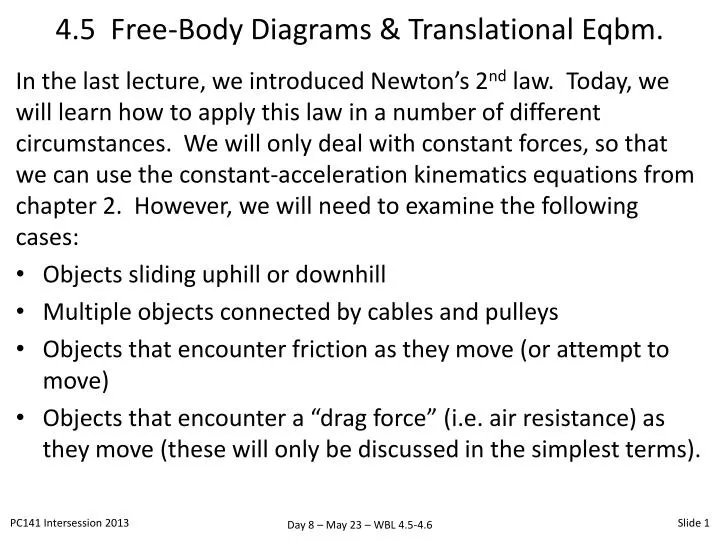
4.5 Free-Body Diagrams & Translational Eqbm. In the last lecture, we introduced Newton’s 2nd law. Today, we will learn how to apply this law in a number of different circumstances. We will only deal with constant forces, so that we can use the constant-acceleration kinematics equations from chapter 2. However, we will need to examine the following cases: • Objects sliding uphill or downhill • Multiple objects connected by cables and pulleys • Objects that encounter friction as they move (or attempt to move) • Objects that encounter a “drag force” (i.e. air resistance) as they move (these will only be discussed in the simplest terms).

4.5 Free-Body Diagrams & Translational Eqbm. Tension When a cable is attached to an object and pulled taut, it pulls on the object with a force that is directed away from the object and along the cable. This force is called tension, often notated . A tension of the same magnitude (but opposite direction) is applied to whatever is causing the pulling. Since the direction of the vector is obvious, we are usually only concerned with finding its magnitude. In this course, we assume cables to be both massless and unstretchable. This greatly facilitates the analysis of problems involving cables, although you don’t need to know why.

4.5 Free-Body Diagrams & Translational Eqbm. Tension and Pulleys In PC141, pulleys are assumed to be massless and frictionless. They exist only as a means to re-direct tension forces along a different direction. • Massless: the rotating pulley does not have any rotational kinetic energy (we’ll come back to that near the end of the course). • Frictionless: refers to the axle; no energy is dissipated during rotation. There is of course a large amount of friction between the cable and the pulley. This is mandatory if they are to move together without slipping. The breaking strength, or simply strength of a cable is the maximum tension that it can withstand before breaking.

4.5 Free-Body Diagrams & Translational Eqbm. Many problems in this chapter are greatly facilitated by drawing a free-body diagram (FBD). Instructions for drawing an FBD are provided on p. 117 of the text. Note that: • Vector arrows do not have to be drawn to scale (in fact, for most problems, you don’t even know the magnitude of all vectors anyhow) • The object or objects that are subjected to forces should not be sketched “photorealistically”. Rather, they should simply be indicated by a small dot or circle. • You should not draw force vectors and acceleration vectors on the same FBD. If you must, then find some way to indicate that the acceleration vectors are “different” (perhaps use a different colour for these vectors)

4.5 Free-Body Diagrams & Translational Eqbm. • Make a sketch (or “space diagram”) of the situation. Often, this will already be provided for you. This is an illustration of the physical situation that you’ve been given. • Isolate the object for which you need to construct a FBD (here, we are concerned with mass 1). At this point, choose the orientation and origin for your axes. It’s best to place the origin at the given position of the object, with the x-axis oriented in the expected direction of travel. In this example, we’re assuming that m1 will slide uphill. If we’re wrong, we will simply get a negative answer for the acceleration. Remember as well that the y-axis must be perpendicular to the x-axis.

4.5 Free-Body Diagrams & Translational Eqbm. • Draw properly-oriented force vectors on the diagram, emanating from the origin (which represents the object). Take care to include ALL possible forces that act on the object. In this case, we have gravity (downward), the normal force (perpendicular to the surface), and tension (along the cable, away from the object, and therefore uphill). Note that the acceleration vector is drawn separately so as to not confuse it with a force vector. • Resolve any forces that are not already directed along x or y into their x- and y-components. Then, write down and solve Newton’s 2nd law in the x- and y-directions. Note that in this particular problem, there can be a positive or negative acceleration along x, but there can not be an acceleration along y, since m1 is confined to the surface.

4.5 Free-Body Diagrams & Translational Eqbm. Now that you know how to produce an FBD, all it takes is practice and repetition in order to master its use. In the class notes and assignments, we will encounter many different problems that require a variety of FBDs in order to solve. In PC141, you will rarely (if ever) have to hand in an FBD for marks, since they’re not easily graded by MasteringPhysics or Scantron. However, you will usually find it necessary to draw one in order to solve your assignment and exam problems. And some advance warning…if you come to my office to request help, my first words will be “show me your FBD”.

4.5 Free-Body Diagrams and Translational Eqbm. Translational Equilibrium As we already know, several forces may act on an objects without producing an acceleration. Since , we can use Newton’s 2nd law to write . With a net force equal to zero, the object either sits at rest or moves with a constant velocity. In 2 dimensions, we can write the condition for translational equilibrium as The text contains 2 very good examples (4.8 and 4.9) that involve translational equilibrium.

Problem #1: Translational Equilibrium WBL LP 4.13

Problem #2: Mowing the Lawn WBL Ex 4.41 A girl pushes a 25-kg lawn mower as shown in the figure. If F = 30 N and = 37°… What is the acceleration of the mower? What is the normal force exerted on the mower by the lawn? Solution: In class

Problem #3: Atwood Machine WBL Ex 4.55 The Atwood machine shown here consists of two masses suspended from a fixed pulley. If m1 = 0.55 kg and m2= 0.80 kg… What is the acceleration of the system of masses? What is the magnitude of the tension in the string? Solution: In class

Problem #4: Inclined Atwood Machine WBL Ex 4.60 In the frictionless inclined Atwood Machine shown here, m1= 2.0 kg. What is m2 if both masses are at rest? What is m2 if both masses are moving at constant velocity? Solution: In class

4.6 Friction Consider the following “thought experiments”… • A book slides across a horizontal surface. The book slows and then stops. This means that the book must have an acceleration parallel to the surface, in the direction opposite to the book’s velocity. • By Newton’s 2nd law, this means that a force must exist in the direction opposite to the book’s velocity. This is the frictional force,. • Now, push horizontally on the book to make it move at a constant velocity. The force that you are applying can not be the only force on the book, otherwise it would be accelerating in the direction of your push. By Newton’s 2nd law, there must be a second force, directed opposite to your push, that exactly balances it. This is also the frictional force,.

4.6 Friction It is tempting to assume that is always oriented in such a way that it opposes the direction of motion. As the walking example in the figure shows, this is not always true. To walk forward, we plant a foot and push backward on the ground with a force . Without friction, the foot would slide backward. With friction, the foot is stationary with respect to the ground (they don’t move relative to each other while they are in contact). This is because is balanced by the equal and opposite force . This proves that friction is, in this case, directed in the direction of motion.

4.6 Friction Here is a second, slightly more complex situation. • In Fig (a), a block rests on a tabletop. As we have seen, there are two forces acting on it; the gravitational force and the normal force . They must be perfectly balanced, since the block is not accelerating. • In Fig. (b), we exert a force on the block, attempting to pull it to the left. In response, a frictional force is directed to the right, balancing so that the block still does not move. is called the static frictional force. • In Figs (c-d), the magnitude of the applied force increases. In response to this, also increases so that the block remains at rest.

4.6 Friction • In Fig (e), the applied force reaches a certain magnitude such that the block begins to slide; for a brief moment it accelerates to the left. The frictional force that opposes this motion is called the kinetic frictional force, . Note that and are not balanced at this moment, which is evident since the block is accelerating. • In response to the onset of motion, you reduce the applied force, as in Fig. (f). When , the block moves at constant velocity. Note that is constant, regardless of the applied force (actually, it’s approximately constant, since the microscopic properties of the surface have a slight variation, as shown on slide 18).

4.6 Friction The text provides this useful figure and graph which explain the same concepts as those from the last 2 slides

4.6 Friction Physical Causes of Friction The frictional force is the vector sum of a vast number of forces acting between the surface atoms of the two objects in contact. If we take two highly-polished (i.e. atomically smooth) and perfectly clean metal surfaces and bring them together in a vacuum (so that no particles are trapped between them), they can cold-weld together instantly, so that no force can cause them to slide apart. This is because the number of atom-to-atom interactions is enormous.

4.6 Friction Frictional Forces and Coefficients of Friction It has been found experimentally that the frictional force (whether static or kinetic) depends critically on the nature of the two surfaces sliding across each other. Also, it appears to be proportional to the normal force that the objects exert on each other. We saw two slides ago that increases in response to an increasing applied force, up until the point where the object starts to slide. Mathematically, we can write the magnitude where is the coefficient of static friction, which depends on the two materials that are sliding against each other(what are the dimensions of this coefficient?)

4.6 Friction Frictional Forces and Coefficients of Friction cont’ The maximum magnitude of static friction is therefore . If all other oppositely-directed forces conspire to exceed this value, then the object starts to slide, as in part (e) of the figure on slide 16. Then, we have a condition of kinetic friction, in which Here, is the coefficient of kinetic friction. Note carefully that the two previous equations are scalar equations, not vector equations. Why must we emphasize this distinction? In general, < . The table on the next slide shows many approximate values of these coefficients.

4.6 Friction

Problem #5: Static Friction on a Level Surface WBL Ex 4.65 A 40-kg crate is at rest on a level surface. If the coefficient of static friction between the crate and the surface is 0.69, what horizontal force is required to get the crate moving? Solution: In class

Problem #6: Static Friction on an Inclined Surface A 40-kg crate is at rest on a surface that can be oriented at any angle. If the coefficient of static friction between the crate and the surface is 0.69 and there are no additional forces other than gravity, what minimum angle must the surface have in order to have the crate begin to slide downhill? Solution: In class

Problem #7: Friction on Inclined Surface WBL Ex 4.79 In the figure, m1 = 2.0 kg and the coefficients of static and kinetic friction between m1and the inclined plane are 0.30 and 0.20, respectively. What is m2 if both masses are at rest? What is m2 if both masses are moving at constant velocity? Solution: In class

4.6 Friction – Air Resistance Air resistance (or “drag”, in general) is a type of friction. Rather than involving surfaces sliding past each other, it occurs when a moving object collides with molecules in a fluid (which can be gas or a liquid…obviously, it’s more of an issue with the latter). Drag depends on the moving object’s size and shape. Minimizing drag when designing an object is the subject of aerodynamics (not part of PC141, or any undergraduate physics course!) it also depends on the moving object’s speed – a fast object encounters more collisions per unit time, leading to a greater amount of drag. A complete mathematical description of drag requires calculus (specifically, differential equations), so we won’t attempt it here. However, we can derive some very simple equations.

4.6 Friction – Air Resistance While small, slow objects experience a drag force that is proportional to their speed v, faster and larger (e.g. human-sized) objects experience a drag force that is proportional to the square of the speed, v2. In all cases, the direction of the drag force f is opposite to that of the velocity. Consider an object that is falling vertically downward. Since drag depends on speed, as the object accelerates downward under the influence of gravity, the drag force – directed upward – will increase. Eventually, the magnitude of the (upward) drag force will equal that of the (downward) gravitational force. At this point, the object can no longer accelerate downward; its velocity will remain constant for the rest of its journey. The value of v at which this occurs is called the terminal velocity, vt. This velocity is a property of the falling object’s shape and size, but also of the density of the fluid through which it is falling.

4.6 Friction – Air Resistance The concept of a terminal velocity can be easily shown using Newton’s 2nd law. For the falling object, . Taking downward as the positive direction, we recall that the two forces present are gravity (downward) and drag (upward). That is, Rearranging, we find that As the object’s velocity increases, so does f. Keeping in mind thatg and m are constant, a point will eventually be reached when f = mg. This implies that acceleration has dropped to zero, and that the object has reached its terminal velocity.

Problem #8: Parachuting WBL LP 4.17

4.5 Free-Body Diagrams & Translational Eqbm .