Download
1 / 42
430 likes | 590 Views
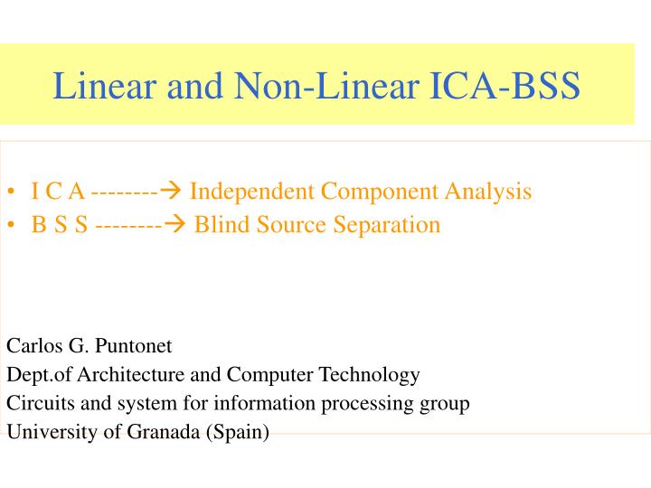
Linear and Non-Linear ICA-BSS. I C A -------- Independent Component Analysis B S S -------- Blind Source Separation Carlos G. Puntonet Dept.of Architecture and Computer Technology Circuits and system for information processing group University of Granada (Spain).

E N D
Linear and Non-Linear ICA-BSS I C A -------- Independent Component Analysis B S S -------- Blind Source Separation Carlos G. Puntonet Dept.of Architecture and Computer Technology Circuits and system for information processing group University of Granada (Spain)
The Problem of “linear” blind separation of p sources: Original signals: s(t)=[s1(t),....,sp(t)]T Mixture: e(t)=[e1(t),...,ep(t)]T Mixture matrix: A(t) pxp The goal is to estimate A(t) by means of W(t) such that the output vector, s*(t) is:
REAL APLICATIONS BSS is Independent Component Analysis (ICA) Noise Elimination in general Speech Processing (Cocktail Party, Noise environment,...) Sonar, Radar Sismic waves Preprocessing recognition Image Processing Biomedicine (ECG, EEG, fMRI,...)
Geometric methods I: Digital * Binary Signals S1u= (1,...,0,...,0)t ..................... Siu= (0,...,1,...,0)t ..................... Spu= (0,...,0,...,1)t The image of a base vector Siu is the vector Aoi, i.e. the column i of the unknown mixture matrix Ao: h(Siu) = Aoi
Geometric methods II: Slopes Slope Function: Extreme values: For input Vectors: aij = min { ei . ej-1 } ej > 0 i,j0{1,..,p}
* Fast method for p=2 signals * Valid for random or bounded sources * Slopes are the independent components * Modifiable for p>2
GENERAL p-DIMMENSIONAL METHOD Obtained matrix W: For p points verifying minimum value of:
* Geometric method for p signals * Valid for random or bounded sources * Slopes are the independent components * No order statistics * Probability of obtaining p points close to the hiper- parallelepiped edges ?
Geometric methods III: Speech • For Linear mixtures • Unimodal p.d.f.’s (non-uniform’s) • Detection of max.density points in the mixture space • Normalization and detection in the sphere radius-unit.
SOURCE SPACE MIXTURE SPACE FROM
NEW GEO-METHOD with KURTOSIS. • (K(e1)>0) and (K(e2)>0) • (K(e1)<0) or (K(e2)<0)
Lattice of Space • M1*M2 Cells. Threshold (TH), and Red-Cells with points > TH.
ICA COMPONENTS FROM KURTOSIS: • If K(e1)>0 and K(e2)>0 Maximum Density Zones • If K(e1)<0 or K(e2)<0 Border Detection
Geometric methods IV: Heuristic + Neural networks Separation of Sources using Simulated Annealing and Competitive Learning Univ. Regensburg and Univ. Granada - New adaptive procedure for the linear and “non-linear” separation - Signals with non-uniform, symmetrical probability distributions - Simulated annealing, competitive learning, and geometric methods - Neural network, and multiple linearization in the mixture space - Simplicity and rapid convergence - Validated by speech signals or biomedical data.
Space Quantization: Observation space with n p-spheres (n=4, p=2)
Simulated Annealing: Energy Function: Fourth-order cumulant : Weights generation:
Simulated Annealing and Competitive Learning 1 0 time SA CL
NON-LINEAR: Contour for where the mixture can be considered linear
Simulation 2: Non-linear mixture of 2 digital 32-valued signals
Simulation 3: EEG signals Eye blink --> Low wave 1 --> Musc. Spik. --> Low wave 2 --> Cardi. Contam. -->
Genetic Algorithms are one of the most popular stochastic optimisation techniques. Inspired by natural genetics and the biological evolutionary process: * A scheme for encoding solutions to a problem in the form of a chromosome (chromosomal representation). · * An evaluation function which indicates the fitness of each chromosome relative to the others in the current set of chromosomes (referred to as population). · * An initialisation procedure for the population of chromosomes. · * A set of parameters that provide the initial settings for the algorithm: the population size and probabilities employed by the genetic operators. *The GA evaluates a given population and generates a new one iteratively, with each successive population referred to as a generation, from genetic operations: reproduction, crossover and mutation.
¡¡¡¡¡ THE END !!!!! THANK YOU VERY MUCH DANKESHÖN GRACIAS