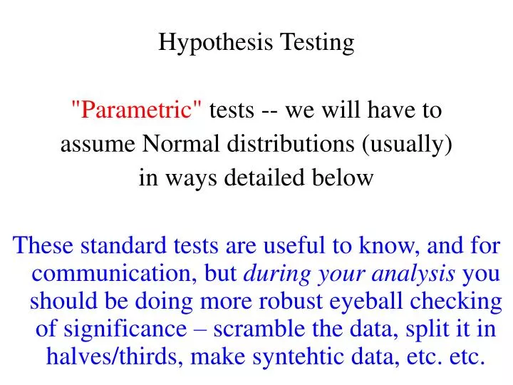
Hypothesis Testing "Parametric" tests -- we will have to assume Normal distributions (usually)

1. Hypothesis Testing • "Parametric" tests -- we will have to • assume Normal distributions (usually) • in ways detailed below • These standard tests are useful to know, and for communication, but during your analysis you should be doing more robust eyeball checking of significance – scramble the data, split it in halves/thirds, make syntehtic data, etc. etc.

2. purpose of the lecture to introduce Hypothesis Testing the process of determining the statistical significance of results

3. Part 1 motivation random variation as a spurious source of patterns

4. d x

5. looks pretty linear d x

6. actually, its just a bunch of random numbers! figure(1); for i = [1:100] clf; axis( [1, 8, -5, 5] ); hold on; t = [2:7]'; d = random('normal',0,1,6,1); plot( t, d, 'k-', 'LineWidth', 2 ); plot( t, d, 'ko', 'LineWidth', 2 ); [x,y]=ginput(1); if( x<1 ) break; end end the script makes plot after plot, and lets you stop when you see one you like

7. the linearity was due to random variation Beware: 5% of random results will be "significant at the 95% confidence level"! The following are "a priori" significance tests. You have to have an a priori reason to be looking for a particular relationship to use these tests properly For a data "fishing expedition" the significance threshold is higher, and depends on how long you've been fishing!

8. Four Important Distributionsused in hypothesis testing

9. #1: the Z distribution(standardized Normal distribution)("Z scores")p(Z) is theNormal distribution for a quantity Z with zero mean and unit variance

10. if d is Normally-distributed with mean d and variance σ2d • then Z = (d-d)/ σd is Normally-distributed with zero mean and unit variance • The "Z score" of a result is just "how many sigma it is from the mean"

11. #2: t-scoresthe distribution of a finite sample (N) of values e that are Z distributed in reality this is a new distribution, called the "t-distribution"

12. t-distribution N=5 p(tN) N=1 tN

13. t-distribution • becomes Normal p.d.f. • for large N N=5 p(tN) • heavier tails than a • Normal p.d.f. • for small N * N=1 tN N=1 • *because you mis-estimate the mean with too few samples, such that values • too far from the mis-estimated mean are far more likely than rapid exp(-x^2) falloff

14. #3 the chi-squared distribution The Normal or Z distribution comes from the limit of the sum of any large number of i.i.d. variables. The chi-squared distribution comes from the sum of the square of N Normally distributed variables. Its limit is therefore Normal, but for N < ∞ it differs... For one thing, it is positive definite!

15. Chi-squared distribution total error • E = χN2 = Σi=1Nei2

16. Chi-squared total error • E = χN2 = Σi=1Nei2 p(E) is called 'chi-squared' when ei is Normally-distributed with zero mean and unit variance called chi-squared p.d.f

17. Chi-Squared p.d.f. the PDF of the sum of squared Normal variables N called “the degrees of freedom” mean N, variance 2N N=1 p(cN2) 2 3 4 5 c2 • asymptotes to • Normal (Gaussian) • for large N

18. In MatLab

19. #4 Distribution of the ratio of two variances from finite samples (M,N) (each of which is Chi-squared distributed) it's another new distribution, called the "F-distribution"

20. F-distribution The ratio of two imperfect (undersampled) estimates of unit variance – for N,M  ∞ it becomes a spike at 1 as both estimates are right • skewed at low N and M N=2 50 p(FN,2) F N=2 50 p(FN,5) F N=2 50 p(FN,25) F N=2 50 p(FN,50) F • starts to look Normal, and gets narrower • around 1 for large N and M

21. Part 4 Hypothesis Testing

22. Step 1. State a Null Hypothesissome version ofthe result is due to random or meaningless data variations(too few samples to see the truth)

23. Step 1. State a Null Hypothesissome variation ofthe result is due to random variation • e.g. • the means of the Sample A and Sample B are different only because of random variation

24. Step 2. Define a standardized quantity that is unlikely to be largewhen the Null Hypothesis is true

25. Step 2. Define a standardized quantity that is unlikely to be largewhen the Null Hypothesis is true • called a “statistic”

26. e.g. • the difference in the means Δm=(meanA – meanB) is unlikely to be large (compared to the standard deviation) if the Null Hypothesis is true

27. Step 3.Calculate that the probability that your observed value or greater of the statistic would occur if the Null Hypothesis were true

28. Step 4.Reject the Null Hypothesisif such large values have a probability of ocurrence ofless than 5% of the time

29. An example test of a particle size measuring device

30. manufacturer's specs: * machine is perfectly calibrated so particle diameters scatter about true value * random measurement error is σd = 1 nm

31. your test of the machine purchase batch of 25 test particles each exactly 100 nm in diameter measure and tabulate their diameters repeat with another batch a few weeks later

32. Results of Test 1

33. Results of Test 2

34. Question 1Is the Calibration Correct? Null Hypothesis: The observed deviation of the average particle size from its true value of 100 nm is due to random variation (as contrasted to a bias in the calibration).

35. in our case = 0.278 and 0.243 the key question is Are these unusually large values for Z ?

36. example for Normal (Z) distributed statistic P(Z’) is the cumulative probability from-∞ to Z’ called erf(Z') p(Z) Z Z’ 0

37. The probability that a difference of either sign between sample means A and B is due to chance isP( |Z| > Zest )This is called a two-sided test p(Z) Z 0 -Zest Zest • which is • 1 – [erf(Zest) - erf(-Zest)]

38. in our case = 0.278 and 0.243 the key question is Are these unusually large values for Z ? = 0.780 and 0.807 So values of |Z| greater than Zest are very common The Null Hypotheses cannot be rejected. There is no reason to think the machine is biased

39. suppose the manufacturer had not specified that random measurement error is σd = 1 nmthen you would have to estimate it from the data = 0.876 and 0.894

40. but then you couldn’t form Zsince you need the true variance

41. we examined a quantity t, defined as the ratio of a Normally-distributed variable e and something that has the form of an estimated standard deviation instead of the true sd:

42. so we will test t instead of Z

43. in our case = 0.297 and 0.247 Are these unusually large values for t ?

44. in our case = 0.297 and 0.247 Are these unusually large values for t ? = 0.768 and 0.806 = 0.780 and 0.807 So values of |t| > test are very common (and verrry close to Z test for 25 samples) The Null Hypotheses cannot be rejected there is no reason to think the machine is biased

45. Question 2Is the variance in spec? Null Hypothesis: The observed deviation of the variance from its true value of 1 nm2 is due to random variation (as contrasted to the machine being noisier than the specs).

46. Results of the two tests = ? the key question is: • Are these unusually large values for χ2 • based on 25 independent samples?

47. Are values ~20 to 25 unusual for a chi-squared statistic with N=25?No, the median almost follows N

48. In MatLab = 0.640 and 0.499 So values of χ2greater than χest2 are very common The Null Hypotheses cannot be rejected there is no reason to think the machine is noiser than advertised

49. Question 3Has the calibration changed between the two tests? Null Hypothesis The difference between the means is due to random variation (as contrasted to a change in the calibration). = 100.055 and 99.951

50. since the data are Normaltheir means (a linear function) are Normaland the difference between them (a linear function) is Normal