Download
1 / 57
570 likes | 707 Views
Loss-based Learning with Latent Variables. M. Pawan Kumar École Centrale Paris École des Ponts ParisTech INRIA Saclay , Île-de-France. Joint work with Ben Packer, Daphne Koller, Kevin Miller and Danny Goodman. Image Classification. Images x i. Boxes h i. Labels y i. Image x.

E N D
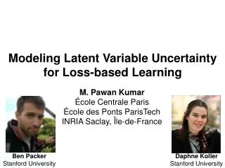
Loss-based Learningwith Latent Variables M. Pawan Kumar ÉcoleCentrale Paris Écoledes PontsParisTech INRIA Saclay, Île-de-France Joint work with Ben Packer, Daphne Koller, Kevin Miller and Danny Goodman
Image Classification Images xi Boxes hi Labels yi Image x Bison Deer Elephant y = “Deer” Giraffe Llama Rhino
Image Classification Feature Ψ(x,y,h) (e.g. HOG) Score f : Ψ(x,y,h) (-∞, +∞) f(Ψ(x,y1,h))
Image Classification Feature Ψ(x,y,h) (e.g. HOG) Score f : Ψ(x,y,h) (-∞, +∞) Prediction y(f) Learn f f(Ψ(x,y1,h)) f(Ψ(x,y2,h))
Loss-based Learning User defined loss function Δ(y,y(f)) f* = argminfΣiΔ(yi,yi(f)) Minimize loss between predicted and ground-truth output No restriction on the loss function General framework (object detection, segmentation, …)
Outline • Latent SVM • Max-Margin Min-Entropy Models • Dissimilarity Coefficient Learning Andrews et al., NIPS 2001; Smola et al., AISTATS 2005; Felzenszwalb et al., CVPR 2008; Yu and Joachims, ICML 2009
Image Classification Images xi Boxes hi Labels yi Image x Bison Deer Elephant y = “Deer” Giraffe Llama Rhino
Latent SVM Scoring function Parameters Features wTΨ(x,y,h) Prediction y(w),h(w) = argmaxy,hwTΨ(x,y,h))
Learning Latent SVM Training data {(xi,yi), i= 1,2,…,n} w* = argminwΣiΔ(yi,yi(w)) Highly non-convex in w Cannot regularize w to prevent overfitting
Learning Latent SVM Training data {(xi,yi), i= 1,2,…,n} wTΨ(x,yi(w),hi(w)) + Δ(yi,yi(w)) - wTΨ(x,yi(w),hi(w)) ≤ wTΨ(x,yi(w),hi(w)) + Δ(yi,yi(w)) - maxhiwTΨ(x,yi,hi) ≤ maxy,h{wTΨ(x,y,h) + Δ(yi,y)} - maxhiwTΨ(x,yi,hi)
Learning Latent SVM Training data {(xi,yi), i= 1,2,…,n} minw ||w||2 + C Σiξi wTΨ(xi,y,h) + Δ(yi,y) - maxhiwTΨ(xi,yi,hi)≤ ξi Difference-of-convex program in w Local minimum or saddle point solution (CCCP) Self-Paced Learning, NIPS 2010
Recap Scoring function wTΨ(x,y,h) Prediction y(w),h(w) = argmaxy,hwTΨ(x,y,h)) Learning minw ||w||2 + C Σiξi wTΨ(xi,y,h) + Δ(yi,y) - maxhiwTΨ(xi,yi,hi)≤ ξi
Image Classification Images xi Boxes hi Labels yi Image x Bison Deer Elephant y = “Deer” Giraffe Llama Rhino
Image Classification Score wTΨ(x,y,h) (-∞, +∞) wTΨ(x,y1,h)
Image Classification Score wTΨ(x,y,h) (-∞, +∞) Only maximum score used No other useful cue? Uncertainty in h wTΨ(x,y1,h) wTΨ(x,y2,h)
Outline • Latent SVM • Max-Margin Min-Entropy (M3E) Models • Dissimilarity Coefficient Learning Miller, Kumar, Packer, Goodman and Koller, AISTATS 2012
M3E Scoring function Partition Function Pw(y,h|x)=exp(wTΨ(x,y,h))/Z(x) Rényi Entropy Marginalized Probability Prediction y(w) = argminy Hα(Pw(h|y,x)) – log Pw(y|x) Gα(y;x,w) RényiEntropy of Generalized Distribution
Rényi Entropy Σh Pw(y,h|x)α 1 Gα(y;x,w) = log 1-α Σh Pw(y,h|x) α = 1. Shannon Entropy of Generalized Distribution - Σh Pw(y,h|x)log(Pw(y,h|x)) Σh Pw(y,h|x)
Rényi Entropy Σh Pw(y,h|x)α 1 Gα(y;x,w) = log 1-α Σh Pw(y,h|x) α = Infinity. Minimum Entropy of Generalized Distribution - maxh log(Pw(y,h|x))
Rényi Entropy Σh Pw(y,h|x)α 1 Gα(y;x,w) = log 1-α Σh Pw(y,h|x) α = Infinity. Minimum Entropy of Generalized Distribution - maxhwTΨ(x,y,h) Same prediction as latent SVM
Learning M3E Training data {(xi,yi), i= 1,2,…,n} w* = argminwΣiΔ(yi,yi(w)) Highly non-convex in w Cannot regularize w to prevent overfitting
Learning M3E Training data {(xi,yi), i= 1,2,…,n} Gα(yi(w);xi,w) + - Gα(yi(w);xi,w) Δ(yi,yi(w)) - Gα(yi(w);xi,w) ≤ Gα(yi;xi,w) + Δ(yi,yi(w)) maxy{Δ(yi,y) ≤ Gα(yi;xi,w) + - Gα(y;xi,w)}
Learning M3E Training data {(xi,yi), i= 1,2,…,n} minw ||w||2 + C Σiξi Gα(yi;xi,w) + Δ(yi,y) – Gα(y;xi,w) ≤ ξi When α tends to infinity, M3E = Latent SVM Other values can give better results
Image Classification Mammals Dataset 271 images, 6 classes 90/10 train/test split 5 folds 0/1 loss
Image Classification HOG-Based Model. Dalal and Triggs, 2005
Motif Finding UniProbe Dataset ~ 40,000 sequences Binding vs. Not-Binding 50/50 train/test split 5 Proteins, 5 folds
Motif Finding Motif + Markov Background Model. Yu and Joachims, 2009
Recap Scoring function Pw(y,h|x)=exp(wTΨ(x,y,h))/Z(x) Prediction y(w) = argminyGα(y;x,w) Learning minw ||w||2 + C Σiξi Gα(yi;xi,w) + Δ(yi,y) – Gα(y;xi,w) ≤ ξi
Outline • Latent SVM • Max-Margin Min-Entropy Models • Dissimilarity Coefficient Learning Kumar, Packer and Koller, ICML 2012
Object Detection Images xi Boxes hi Labels yi Image x Bison Deer Elephant y = “Deer” Giraffe Llama Rhino
Minimizing General Loss Supervised Samples minwΣiΔ(yi,hi,yi(w),hi(w)) Weakly Supervised Samples + ΣiΔ’(yi,yi(w),hi(w)) Unknown latent variable values
Minimizing General Loss minwΣiΔ(yi,hi,yi(w),hi(w)) Σhi Pw(hi|xi,yi) A single distribution to achieve two objectives
Problem Model Uncertainty in Latent Variables Model Accuracy of Latent Variable Predictions
Solution Use two different distributions for the two different tasks Model Uncertainty in Latent Variables Model Accuracy of Latent Variable Predictions
Solution Use two different distributions for the two different tasks Pθ(hi|yi,xi) hi Model Accuracy of Latent Variable Predictions
Solution Use two different distributions for the two different tasks Pθ(hi|yi,xi) hi Pw(yi,hi|xi) (yi,hi) (yi(w),hi(w))
The Ideal Case No latent variable uncertainty, correct prediction Pθ(hi|yi,xi) hi hi(w) Pw(yi,hi|xi) (yi,hi(w)) (yi,hi)
In Practice Restrictions in the representation power of models Pθ(hi|yi,xi) hi Pw(yi,hi|xi) (yi,hi) (yi(w),hi(w))
Our Framework Minimize the dissimilarity between the two distributions Pθ(hi|yi,xi) hi User-defined dissimilarity measure Pw(yi,hi|xi) (yi,hi) (yi(w),hi(w))
Our Framework Minimize Rao’s Dissimilarity Coefficient Pθ(hi|yi,xi) hi ΣhΔ(yi,h,yi(w),hi(w))Pθ(h|yi,xi) Pw(yi,hi|xi) (yi,hi) (yi(w),hi(w))
Our Framework Minimize Rao’s Dissimilarity Coefficient Pθ(hi|yi,xi) hi Hi(w,θ) - β Σh,h’Δ(yi,h,yi,h’)Pθ(h|yi,xi)Pθ(h’|yi,xi) Pw(yi,hi|xi) (yi,hi) (yi(w),hi(w))
Our Framework Minimize Rao’s Dissimilarity Coefficient Pθ(hi|yi,xi) hi Hi(w,θ) - β Hi(θ,θ) - (1-β) Δ(yi(w),hi(w),yi(w),hi(w)) Pw(yi,hi|xi) (yi,hi) (yi(w),hi(w))
Our Framework Minimize Rao’s Dissimilarity Coefficient Pθ(hi|yi,xi) hi minw,θ Σi Hi(w,θ) - β Hi(θ,θ) Pw(yi,hi|xi) (yi,hi) (yi(w),hi(w))
Optimization minw,θΣiHi(w,θ) - β Hi(θ,θ) Initialize the parameters to w0 and θ0 Repeat until convergence Fix w and optimize θ Fix θ and optimize w End
Optimization of θ minθΣiΣhΔ(yi,h,yi(w),hi(w))Pθ(h|yi,xi) - β Hi(θ,θ) Pθ(hi|yi,xi) hi hi(w) Case I: yi(w) = yi
Optimization of θ minθΣiΣhΔ(yi,h,yi(w),hi(w))Pθ(h|yi,xi) - β Hi(θ,θ) Pθ(hi|yi,xi) hi hi(w) Case I: yi(w) = yi
Optimization of θ minθΣiΣhΔ(yi,h,yi(w),hi(w))Pθ(h|yi,xi) - β Hi(θ,θ) Pθ(hi|yi,xi) hi Case II: yi(w) ≠ yi
Optimization of θ minθΣiΣhΔ(yi,h,yi(w),hi(w))Pθ(h|yi,xi) - β Hi(θ,θ) Stochastic subgradient descent Pθ(hi|yi,xi) hi Case II: yi(w) ≠ yi
Optimization of w minwΣiΣhΔ(yi,h,yi(w),hi(w))Pθ(h|yi,xi) Expected loss, models uncertainty Form of optimization similar to Latent SVM Concave-Convex Procedure (CCCP) Δ independent of h, implies latent SVM
Object Detection Train Input xi Output yi Input x Bison Deer Elephant Output y = “Deer” Latent Variable h Giraffe Mammals Dataset Llama 60/40 Train/Test Split 5 Folds Rhino