Download

1 / 38
390 likes | 572 Views
Population Review. Exponential growth. N t+1 = N t + B – D + I – E Δ N = B – D + I – E For a closed population Δ N = B – D. dN/dt = B – D B = bN ; D = dN (b and d are instanteous birth and death rates) dN/dT = (b-d)N dN/dt = rN 1.1 N t = N o e rt 1.2.

E N D
Exponential growth • Nt+1 = Nt + B – D + I – E • ΔN = B – D + I – E For a closed population • ΔN = B – D
dN/dt = B – D • B = bN ; D = dN (b and d are instanteous birth and death rates) • dN/dT = (b-d)N • dN/dt = rN 1.1 • Nt = Noert 1.2
Doubling time • Nt = 2 No • 2No = Noer(td) (td = doubling time) • 2 = er(td) • ln(2) = r(td) • td = ln(2) / r 1.3
Assumptions • No I or E • Constant b and d (no variance) • No genetic structure (all are equal) • No age or size structure (all are equal) • Continuous growth with no time lags
Discrete growth • Nt+1 = Nt + rdNt(rd = discrete growth factor) • Nt+1 = Nt(1+rd) • Nt+1 = λ Nt • N2 = λ N1 = λ (λ No) = λ2No • Nt = λtNo 1.4
r vs λ • er = λ if one lets the time step approach 0 • r = ln(λ) • r > 0 ↔ λ > 1 • r = 0 ↔λ = 1 • r < 0 ↔ 0 < λ < 1
Environmental stochasticity • Nt = Noert ; where Nt and r are means σr2 > 2r leads to extinction
Demographic stochasticity • P(birth) = b / (b+d) • P(death) = d / (b+d) • Nt = Noert (where N and r are averages) • P(extinction) = (d/b)^No
Elementary Postulates • Every living organism has arisen from at least one parent of the same kind. • In a finite space there is an upper limit to the number of finite beings that can occupy or utilize that space.
Think about a complex model approximated by many terms in a potentially infinite series. Then consider how many of these terms are needed for the simplest acceptable model. dN/dt = a + bN + cN2 + dN3 + .... From parenthood postulate, N = 0 ==> dN/dt = 0, therefore a = 0. Simplest model ===> dN/dt = bN, (or rN, where r is the intrinsic rate of increase.)
Logistic Growth There has to be a limit. Postulate 2. Therefore add a second parameter to equation. dN/dt = rN + cN2 define c = -r/K dN/dt = rN ((K-N)/K)
Logistic growth • dN/dT = rN (1-N/K) or rN / ((K-N) / K) • Nt = K/ (1+((K-No)/No)e-rt)
Further Refinements of the theory • Third term to equation? • More realism? Symmetry? • No reason why the curve has to be a symmetric curve with maximal growth at N = K/2.
What if the population is too small? Is r still high under these conditions? • Need to find each other to mate • Need to keep up genetic diversity • Need for various social systems to work
Examples of small population problems • Whales, Heath hens, Bachmann's warbler • dN/dt = rN[(K-N)/K][(N-m)/N]
Instantaneous response is not realistic • Need to introduce time lags into the system • dN/dt = rNt[(K-Nt-T)/K]
Three time lag types Monotonic increase of decrease: 0 < rT < e-1 Oscillations damped: e-1 < rT < /2 Limit cycle: rT > /2
1. Nt+1 = Ntexp[r(1-Nt/K)] 2. Nt+1 = Nt[1+r(1-Nt/K)] May, 1974. Science
Logistic growth with difference equations, showing behavior ranging from single stable point to chaos • Nt+1 = Ntexp[r(1-Nt/K)] • Nt+1 = Nt[1+r(1-Nt/K)]
Added Assumptions • Constant carrying capacity • Linear density dependence