COMP 2402/2002

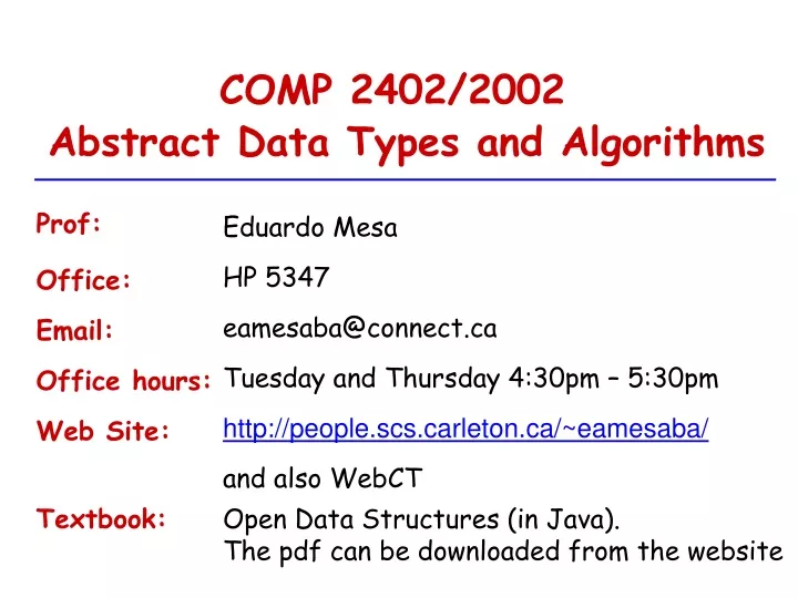
1. COMP 2402/2002 Abstract Data Types and Algorithms Prof: Eduardo Mesa HP 5347 Office: eamesaba@connect.ca Email: Tuesday and Thursday 4:30pm – 5:30pm Office hours: http://people.scs.carleton.ca/~eamesaba/ Web Site: and alsoWebCT Textbook: Open Data Structures (in Java). Thepdf can bedownloadedfromthewebsite

2. TAs Andrew Trenholm Tawfic Abdul-Fatah • No office hours for TAs • Prompt answer to questions in: • Web-CT discussion • Carleton Computer Science Society forum.

3. Evaluation Assignments 30% 3 assignments 10% each Midterm: 30% 2 Midterms 15% each Final Exam: 40% Active Participation: 5% bonus

4. Assignments No late assignment will be accepted. • 1 Theory assignment • Must be handled first thing in class. • All pages must be stapled • 2 Programming Assignments • Must be uploaded on Web CT • Make a folder • (<Student ID>_<First Name>_<Last Name>_ <Assignment #>) • Put all the source files in the folder • Add a text file with your Id and full name • Zip the folder

5. End of theIntroduction Begining of theLecture

6. Data Type a data storage format that can contain a specific type or range of values characterized by a set of operations that satisfy a set of specific properties.

7. Example Data Type Int • Range of Value: -(231) to (231) • Operations: +, -, *, / • Properties: • Symmetry: a+b = b+a, a*b = b*a • Associativea+(b+c) = (a+b)+c • Definition: a/b , b must not be 0

8. Data Structures How to organize data to be able to perform operations on those data efficiently. A variable is the simplest data structure.

9. Example Electronic Phone Book • Contains different DATA: • -Names • - phone numbers • - addresses • Need to perform certain OPERATIONS: • -add • - delete • - look for a phone number • - look for an address

10. Example Electronic Phone Book How to organize the data so to optimize the efficiency of the operations List Binary Search Tree Dictionary A B X Z

11. Example Finding the best route for an email message in a network • Contains DATA: • - Network + Traffic • Need to perform certain OPERATIONS: • - Find the best route 10 12 43 8 7 16 21 9 14 18

12. Example Electronic Phone Book How to represent the data Adjacency Matrix Adjacency List

13. Abstract Data Type (ADT) (interfaces) Define what operation can be done. Implementations (algorithms) Define how each operation is performed. A same ADT could have several different implementations.

14. ADT (Shelf) Peter Lucy GetBook ( Book b ) Random Search Binary Search

15. Data Structures So to perform the operations efficiently we need: • Identify your data • Identify the operationsyou need to perform (and how often each operation is performed) • Defineefficiency • Choose the best structure for your data.

16. Analysis of Algorithms Input Algorithm Output An algorithm is a step-by-step procedure for solving a problem in a finite amount of time. Analyze an algorithm = determine its efficiency

17. Efficiency ? Running time … Memory … Quality of the result …. Simplicity …. Generally, while improving the efficiency in one of these aspects we diminish the efficiency in the others

18. Best case Average case Worst case 120 100 80 Running Time 60 40 20 0 1000 2000 3000 4000 Input Size Running time The running time depends on the input size It also depends on the input data: Different inputs can have different running times

19. Running Time of an algorithm • Average case time is often difficult to determine. • We focus on the worst case running time. • Easier to analyze • Crucial to applications such as games, finance and robotics

20. 15 15 4 10 Example …. If x is odd return x If x is even compute the sum S of the first x integers return S

21. Measuring the Running Time • How should we measure the running time of an algorithm? • Approach 1: Experimental Study

22. Beyond Experimental Studies • Experimental studies have several limitations: • need toimplement • limited set ofinputs • hardware and software environments.

23. Theoretical Analysis • We need a general methodology that: - Uses a high-level description of the algorithm (independent of implementation). Characterizes running time as a function of the input size. Takes into account all possible inputs. Is independent of the hardware and software environment.

24. Analysis of Algorithms • Primitive Operations:Low-level computations independent from the programming language can be identified in pseudocode. • Examples: • calling a method and returning from a method • arithmetic operations (e.g. addition) • comparing two numbers, etc. By inspecting the pseudo-code, we can count the number of primitive operations executed by an algorithm.

25. Example: Algorithm arrayMax(A, n):Input: An array A storing n integers.Output: The maximum element in A.currentMax A[0]fori 1to n -1 doif currentMax < A[i] then currentMax  A[i]return currentMax

26. A 5 13 4 7 6 2 3 8 1 2 currentMax currentMax A[0]fori 1 to n -1 doif currentMax < A[i] then currentMax  A[i] return currentMax

27. A 5 13 4 7 6 2 3 8 1 2 5 currentMax currentMax A[0]fori 1 to n -1 doif currentMax < A[i] then currentMax  A[i] return currentMax

28. A 5 13 4 7 6 2 3 8 1 2 5 currentMax currentMax A[0]fori 1 to n -1 doif currentMax < A[i] then currentMax  A[i] return currentMax

29. What are the primitive operations to count ? A 5 13 4 7 6 2 3 8 1 2 Comparisons Assignments to currentMax 13 currentMax currentMax A[0]fori 1 to n -1 doif currentMax < A[i] then currentMax  A[i] return currentMax

30. 1 assignment n-1 comparisons n-1 assignments (worst case) 5 7 8 10 11 12 14 16 17 20 currentMax A[0]fori 1 to n -1 doif currentMax < A[i] then currentMax  A[i] return currentMax

31. 1 assignment n-1 comparisons 0 assignments 15 1 12 3 9 7 6 4 2 2 In the best case ? currentMax A[0]fori 1 to n -1 doif currentMax < A[i] then currentMax  A[i] return currentMax

32. Summarizing: Worst Case: n-1 comparisons n assignments Best Case: n-1 comparisons 1 assignment Compute the exact number of primitive operations could be difficult We compare the asymptotic behaviour of the running time when the size of the input rise.

33. c • g(n) f(n) n0 n Big-Oh (upper bound) • given two functions f(n) and g(n), we say that f(n) is O(g(n)) if and only if there are positive constants c and n0 such that f(n) c g(n)for n n0

34. 3 g(n) = 3 n What does it mean c g(n) ? • 2 g(n) = 2 n Example: • g(n) = n n n 34

35. g(n) = n2 Graphical example … • f(n) = 2n+1 ? • f(n) is O(n2) n • f(n) c g(n)for n n0 c = 1 n0≈2.5

36. But also • f(n) = 2n+1 • g(n) = n n • f(n) c g(n)for n n0

37. But also • f(n) = 2n+1 • 2 g(n) = 2 n n • f(n) c g(n)for n n0

38. But also • f(n) = 2n+1 • 3 g(n) = 3 n • f(n) is O(n) • c = 3 and n0= 1 n • f(n) c g(n)for n n0

39. 4n 3n 2n On the other hand… n2 is not O(n) because there is no c and n0 such that: n2cn for nn0 ( no matter how large a c is chosen there is an n big enough (n > c) that n2 > c n). n2 n n0 n

40. Notice: O(g(n)) is a set of functions • When we say f(n) = O(g(n)) we really mean f(n)ϵO(g(n)) • Formal definition of big-Oh: • O(g(n)) = {f(n) : there exists positive constants c and n0 • such that f(n) cg(n)for all n n0 }

41. Example: Prove that f(n) = 60n2 + 5n + 1 is O(n2) We must find a constant c and a constant n0 such that: 60n2 + 5n + 1 ≤ c n2for all n≥n0 5n ≤ 5n2for all n≥1 f(n) ≤ 60n2 +5n2 + n2for all n≥1 1 ≤ n2for all n≥1 f(n) ≤ 66n2for all n≥1 c= 66 et n0=1 => f(n) = O(n2)

42. Example: Prove f(n) = 5n log2 n + 8n - 200 = O(n log2 n) 5n log2 n + 8n - 200 ≤ 5n log2 n + 8n ≤ 5n log2 n + 8n log2 n for n ≥ 2 (log2 n ≥ 1) ≤ 13n log2 n f(n) ≤ 13n log2 n for all n ≥ 2 f(n)ϵ O(n log2 n ) [ c = 13, n0 = 2 ]

43. Some commons relations O(nc1) ⊂O(nc2) for any c1 < c2 For any constants a; b; c > 0, O(a)⊂O(log n) ⊂ O(nb) ⊂ O(cn) These make things faster 2 log2 n + 2 = O(log n) n + 2 = O(n) 2n + 15n1/2= O(n) We can multiply these to learn about other functions, O(an) = O(n) ⊂ O(n log n) ⊂ O(n1+b) ⊂ O(ncn) Examples: O(n1/5) ⊂ O(n1/5 log n)

44. Theorem: If g(n)is O(f(n)) , then for any constant c > 0 g(n)is also O(c f(n)) Theorem: O(f(n) + g(n)) = O(max(f(n), g(n))) Ex 1: 2n3 + 3n2= O (max(2n3, 3n2)) = O(2n3) = O(n3) Ex 2: n2 + 3 log n – 7 = O(max(n2, 3 log n – 7)) = O(n2)

45. Simple Big Oh Rule: • Drop lower order terms and constant factors • 7n-3 is O(n) • 8n2log n + 5n2 + n is O(n2log n) • 12n3 + 5000n2 + 2n4 is O(n4)

46. Other Big Oh Rules: • Use the smallest possible class of functions • Say “2n is O(n)” instead of “2n is O(n2)” • Use the simplest expression of the class • Say “3n+5 is O(n)” instead of • “3n+5 is O(3n)”

47. Asymptotic Notation (terminology) • Special classes of algorithms: constant: O(1) logarithmic: O(log n) linear: O(n) quadratic: O(n2) cubic: O(n3) polynomial: O(nk), k >0 exponential: O(an), n > 1

48. 5 9 7.3 7.5 … … … … … … Example of Asymptotic Analysis An algorithm for computing prefix averages The i-th prefix average of an array X is average of the first (i+ 1)elements of X X[0] +X[1] +… +X[i] A[i]= (i+ 1) 5 13 4 8 6 2 3 8 1 2

49. Example of Asymptotic Analysis AlgorithmprefixAverages1(X, n) Inputarray X of n integers Outputarray A of prefix averages of X #operations A new array of n integers fori0ton  1do sX[0] forj1toido ss + X[j] A[i]s / (i + 1) returnA

50. i 5 5 13 4 8 6 2 3 8 1 2 j = 0