Download
1 / 26
260 likes | 380 Views
Macroeconomics Prof. Juan Gabriel Rodríguez. Chapter 4 The IS-LM Model. Question. How is output and interest rate determined simultaneously in the short run?

E N D
MacroeconomicsProf. Juan Gabriel Rodríguez Chapter 4 The IS-LM Model
Question How is output and interest rate determined simultaneously in the short run? Output and the interest rate are determined by simultaneous equilibrium in the goods and money markets. In the short run, we assume that production responds to demand without changes in price (i.e., price is fixed), so output is determined by demand. [The interest rate affects output (through investment) and output affects the interest rate (through money demand), so it is necessary to consider the simultaneous determination of output and the interest rate]
The demand for goods is: Z = C(Y-T) + I + G Consumption: linear. Investment (I): exogenous. Government Spending (G): exogenous. No role for the interest rate The Goods Market: the IS Relation
The Goods Market: the IS Relation In equilibrium: Y = C(Y-T) + I + G Now, investment will depend on: • The level of sales (Y): + • The interest rate (i + x): - I = I(Y,i+x) x: external finance premium, the premium the bank asks for loans that are not guaranteed by firm’s capital
The Goods Market: the IS Relation x depends on: 1. Bank’s capital (AB): a fall in the bank’s capital (bank’s clients fail to pay their loans back) increases leverage. To restore the original leverage ratio, the bank can decrease assets (reduction of loans –first reaction!) or increase capital (look for new investors) 2. Firm’s capital (AF): this capital is used as a guarantee for the loan. It also determines the firm’s incentives to choose investment projects (the larger AF, the more the firm has to lose if the project fails) Therefore, x=x(AB,AF)
The Goods Market: the IS Relation Taking into account the investment relation, the equilibrium condition in the goods market becomes: Y = C(Y-T) + I(Y,i+x) + G • For a given value of the interest rate i+x, demand is an increasing function of output, for two reasons: • An increase in output leads to an increase in income and also to an increase in disposable income. • An increase in output also leads to an increase in investment.
The Goods Market: the IS Relation Two characteristics of Z: • Because it’s assumed that the consumption and investment relations are not linear, Z is, in general, a curve rather than a line. • Z is drawn flatter than a 45-degree line because it’s assumed that an increase in output leads to a less than one-for-one increase in demand.
The Goods Market: the IS Relation Production Z,Y (Production) Z Equilibrium output is determined by the condition that production be equal to demand. Equilibrium point Y (Income)
The Goods Market: the IS Relation Z,Y An increase in i decreases the demand for goods at any level of output, leading to a decrease in the equilibrium level of output. Equilibrium in the goods market implies that an increase in the interest rate leads to a decrease in output. The IS curve is therefore downward sloping. Production Z Z’ Equilibrium point Y i i’ i IS curve Y’ Y Y
The Goods Market: the IS Relation • We have drawn the IS curve, taking as given the values of taxes, T, and government spending, G. Changes in either T or G will shift the IS curve. • In particular: • Changes in factors that decrease the demand for goods, given the interest rate, shift the IS curve to the left. • Changes in factors that increase the demand for goods, given the interest rate, shift the IS curve to the right.
The Goods Market: the IS Relation i An increase in taxes shifts the IS curve to the left. i What about x? IS IS’ Y’ Y Y
The Goods Market: the IS Relation x Investment expenditure Spreads x
The Finantial Market: the LM Relation The interest rate is determined by the equality of the supply of and the demand for money: M = €YL(i) M = nominal money stock€YL(i) = demand for money€Y = nominal incomei = nominal “interest” rate
The Finantial Market: the LM Relation The LM relation: In equilibrium, the real money supply is equal to the real money demand, which depends on real income, Y and i: Recall that Nominal GDP = Real GDP multiplied by the GDP deflator: €Y=YP Equivalently: €Y/P=Y
The Finantial Market: the LM Relation i An increase in income leads, at a given interest rate, to an increase in the demand for money. Given the money supply, this increase in the demand for money leads to an increase in the equilibrium interest rate. Ms i’ i Md’ (Y’) Md (Y) M/P M i Equilibrium in the financial markets implies that an increase in income leads to an increase in the interest rate. The LM curve is therefore upward sloping. LM i’ i Y Y’ Y
The Finantial Market: the LM Relation An increase in money causes the LM curve to shift down. i i LM LM’ i i’ Y Y
The IS-LM Model IS RelationY = C(Y-T) + I(Y,i+x) +G Equilibrium in the goods market implies that an increase in the interest rate leads to a decrease in output. This is represented by the IS curve. Equilibrium in financial markets implies that an increase in output leads to an increase in the interest rate. This is represented by the LM curve. Only at the point where both curves cross, are both goods and financial markets in equilibrium. i LM i IS Y Y
The IS-LM Model i LM Taxes affect the IS curve, not the LM curve. Fiscal Contraction (reduction in G or increase in T) Spread x (reduction of AB or/and AF) i i’ IS IS’ Y’ Y Y
The IS-LM Model i Monetary policy does not affect the IS curve, only the LM curve. LM LM’ A monetary expansion leads to higher output and a lower interest rate. i i’ IS Y Y’ Y
The IS-LM Model Investment = Private saving + Public saving I = S + (T – G) A fiscal contraction may decrease investment. Or, looking at the reverse policy, a fiscal expansion—a decrease in taxes or an increase in spending—may actually increase investment.
The IS-LM Model • The combination of monetary and fiscal polices is known as the monetary-fiscal policy mix, or simply, the policy mix. • Sometimes, the right mix is to use fiscal and monetary policy in the same direction. • Sometimes, the right mix is to use the two policies in opposite directions—for example, combining a fiscal contraction with a monetary expansion...
The IS-LM Model: an example The U.S. Growth Rate, 1999:1 to 2002:4
The IS-LM Model: an example Monetary policy: The Federal Funds Rate, 1999:1 to 2002:4
The IS-LM Model: an example Fiscal policy: U.S. Federal Government Revenues and Spending (as Ratios to GDP), 1999:1 to 2002:4
The IS-LM Model: an example i Sharp decline in investment demand: there were extremely optimistic expectations in the period previous to the recession LM LM’ E i i’ • Expansion of the money supply: LM to LM’ • Expansion of public spending and reduction in tax rates: IS’ to IS’’ E’’ E’ i’’ IS IS’’ IS’ Y’ Y’’ Y Y
The IS-LM Model: an example - The policy (monetary and fiscal) decreased both the depth and the length of the recession, but it was not enough to avoid the recession… Dynamics: Time is needed for output to adjust to changes in fiscal and monetary policy • Consumers are likely to take some time to adjust their consumption following a change in disposable income. • Firms are likely to take some time to adjust investment spending following a change in their sales. • Firms are likely to take some time to adjust investment spending following a change in the interest rate. • Firms are likely to take some time to adjust production following a change in their sales.