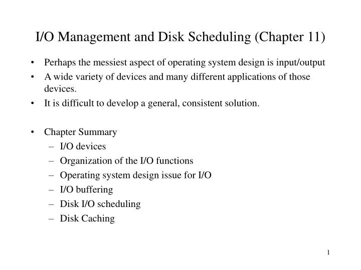
I/O Management and Disk Scheduling (Chapter 11)

1. I/O Management and Disk Scheduling (Chapter 11) • Perhaps the messiest aspect of operating system design is input/output • A wide variety of devices and many different applications of those devices. • It is difficult to develop a general, consistent solution. • Chapter Summary • I/O devices • Organization of the I/O functions • Operating system design issue for I/O • I/O buffering • Disk I/O scheduling • Disk Caching

2. I/O Devices • External devices that engage in I/O with computer systems can be roughly grouped into three categories: • Human readable: Suitable for communicating with the computer user. Examples include printers, video display terminals, consisting of display, keyboard, and mouse. • Machine readable: Suitable for communicating with electronic equipment. Examples are disk and tape drives, sensors, controllers, and actuators (devices which transform an input signal (mainly an electrical signal) into motion). • Communication: Suitable for communicating with remote devices. Examples are digital line drivers and modems.

3. Differences across classes of I/O • Data rate: See Figure 11.1. • Application: The use to which a device is put has an influence on the software and policies in the O.S. and supporting utilities. For example: • A disk used for files requires the support of file-management software. • A disk used as a backing store for pages in a virtual memory scheme depends on the use of virtual memory hardware and software. • A terminal can be used by the system administrator or regular user. These uses imply different levels of privilege and priority in the O.S.

5. Differences across classes of I/O (continue) • Complexity of control: A printer requires a relatively simple control interface. A disk is much more complex. • Unit of transfer: Data may be transferred as a stream of bytes or characters (e.g., terminal I/O) or in large blocks (e.g., disk I/O). • Data representation: Different data-encoding schemes are used by different devices, including differences in character code and parity conventions. • Error conditions: The nature of errors, the way in which they are reported, their consequences, and the available range of responses differ widely from one device to another.

6. Organization of the I/O Function • Programmed I/O: The processor issues an I/O command on behalf of a process to an I/O module; that process then busy-waits for the operation to be completed before proceeding. • Interrupt-driven I/O: The processor issues an I/O command on behalf of a process, continues to execute subsequent instructions, and is interrupted by the I/O module when the latter has completed its work. The subsequent instructions may be in the same process if it is not necessary for that process to wait for the completion of the I/O. Otherwise, the process is suspended pending the interrupt, and other work is performed. • Direct memory access (DMA): A DMA module controls the exchange of data between main memory and an I/O module. The processor sends a request for the transfer of a block of data to the DMA module and is interrupted only after the entire block has been transferred.

8. The Evolution of the I/O Function • The processor directly controls a peripheral device. This is seen in simple microprocessor-controlled devices. • A controller or I/O module is added. The processor uses programmed I/O without interrupts. With this step, the processor becomes somewhat divorced from the specific details of external device interfaces. • The same configuration as step 2 is used, but now interrupts are employed. The processor need not spend time waiting for an I/O operation to be performed, thus increasing efficiency. • The I/O module is given direct control of memory through DMA. It can now move a block of data to or from memory without involving the processor, except at the beginning and end of the transfer.

10. The Evolution of the I/O Function (cont.) • I/O channel: The I/O module is enhanced to become a separate processor with a specialized instruction set tailored for I/O. The central processor unit (CPU) directs the I/O processor to execute an I/O program in main memory. The I/O processor fetches and executes these instructions without CPU intervention. This allows the CPU to specify a sequence of I/O activities and to be interrupted only when the entire sequence has been performed. • I/O processor: The I/O module has a local memory of its own and is, in fact, a computer in its own right. With this architecture, a large set of I/O devices can be controlled with minimal CPU involvement. A common use for such an architecture has been to control communications with interactive terminals. The I/O processor takes care of most of the tasks involved in controlling the terminals.

11. Operating System Design Issues • Design Objectives: Efficiency and Generality • Efficiency • I/O is often the bottleneck of the computer system. • I/O devices are slow • Use multi-programming (process1 is put on wait and process2 goes to work) • Main memory limitation => all process in main memory waiting for I/O • Bringing in more processes => more I/O operations • Virtual memory => partially loaded processes, swapping on demand • The design of I/O for greater efficiency: optimize Disk I/O • hardware & scheduling policies • Generality • For simplicity & freedom from error, it is desirable to handle all devices in a uniform manner. • Hide most details and interact through general functions: Read, Write, Open, Close, Lock, Unlock.

12. Logical Structure of the I/O Function • Logical I/O: Concerned with managing general I/O functions on behalf of user processes, allowing them to deal with the device in terms of a device identifier and simple commands: Open, Close, Read, and Write. • Device I/O: The requested operations and data are converted into appropriate sequences of I/O instructions, channel commands, and controller orders. Buffering techniques may be used to improve utilization. • Scheduling and control: The actual queuing and scheduling of I/O operations occurs at this level. Interrupts are handled and I/O status is reported. This is the software layer that interacts with the I/O module and the device hardware. • Directory management: Symbolic file names are converted to identifiers. This level is also concerned with user operations that affect the directory of files, such as Add, Delete, and Reorganize. • File system: Deals with logical structure of files. Open, Close, Read, Write. Access rights are handled in this level. • Physical organization: References to files are converted to physical secondary storage addresses, taking into account the physical track and sector structure of the secondary storage device. Allocation of secondary storage space and main storage buffers is handled in this level.

13. e.g., TCP/IP e.g., keyboard, mouse

14. I/O Buffering • Objective: To improve system performance by buffering • Methods: • To perform input transfers in advance of the requests being made; • To perform output transfers some time after the request is made; • Two types of I/O devices • Block-oriented: • Store information in blocks that are usually of fixed size. • Transfers are made a block at a time. • E.g., tapes and disks. • Stream-oriented: • Transfer data in and out as a stream of bytes. • There is no block structure. • E.g., terminals, printers, communication ports, mouse, other pointing devices, most other devices that are not secondary storage.

15. Main memory Program Data Program Data I/O device Process1 Process1 I/O request (read) Transfer data block Writing a data block to an I/O device Data area for I/O Data area for I/O Reading a data block from an I/O device Main memory I/O device I/O request (write) Transfer data block Process, main memory and I/O device • Reading and writing a data block from and to an I/O device may cause single process deadlock. • When the process invokes an I/O request, the process will be blocked on this I/O event. • Suppose the OS swaps this process out of the main memory. • When the data from the I/O device is ready for transfer, the I/O device must wait for the process to be swapped back into the main memory. • The OS is very unlikely to swap this process back into the main memory because this process is still being blocked. Hence a deadlock occurs. • Remedy: • Lock up the data area for I/O in the main memory. Swapping of this part is not allowed. • A better solution is to have a buffer area for I/O in the main memory.

16. Operations of buffering schemes • No buffering • I/O device transfers data to user space of process. • The process performs processing on the data. • Upon completion of the processing, the process asks for the next data transfer from the I/O device. • Single buffer • Buffer size: a character, a line, or a block • Operations: • Input transfer made to buffer. • Upon completion of transfer, the process moves the block into user space. • The process immediately requests another block (read ahead). • Efficiency is achieved because while the process is processing the first block, the next block is being transferred. • Data output is similar. • For most of the time, this second block will be used by the process. • Similar to single-buffer producer-consumer model in Chapter 5. • Double buffer • A process transfers data to (or from) one buffer while the I/O device works on the other buffer. • Circular buffer • Extends double buffer case by adding more buffers. • Good for processes with rapid bursts of I/O. • Similar to bounded-buffer producer-consumer model in Chapter 5.

18. The utility of Buffering • The buffers are always in the OS system memory space, which are always locked. Thus an entire process can be swapped out without worrying about single process deadlock. • Buffering is a technique that smoothes out peaks in I/O demand. • No amount of buffering will allow an I/O device to keep pace indefinitely with a process when the average demand of the process is greater than the I/O device can service. • All buffers will eventually fill up and the process will have to wait after processing each block of data. • In a multiprogramming environment, when there is a variety of I/O activities and a variety of process activities to service, buffering is one of the tools that can increase the efficiency of the OS and the performance of individual processes.

19. Disk I/O • The speed of CPUs and main memory has far outstripped that of disk access. The disk is about four orders of magnitude slower than main memory (Fig 11.1). • Disk Performance Parameters: • Seek time • Seek time is the time required to move the disk arm to the required track. • Seek time consists of two components: • the initial startup time • The time taken to traverse the tracks that have to be crossed once the access arm is up to speed. • For a typical 3.5-inch hard disk, the arm may have to traverse up to slightly less than 3.5/2 = 1.75 inches. • The traverse time is not a linear function of the number of tracks. • Typical average seek time: < 10 milliseconds (msec or ms) • Ts = m X n + s where Ts = seek time, n = # of tracks traversed, m is a constant depends on the disk drive, and s = startup time.

21. Track

22. Disk I/O (continue) • Rotational delay (or rotational latency) • Disks, other than floppy disks, rotate at 5400 to 15000 rpm, which is one revolution per 11.1 msec to 4 msec. • 15000 rpm <=> 250 rps => 1 rotation takes 1/250 = 4 msec • On the average, the rotational delay will be 2 msec for a 15000 rpm HD. • Floppy disks rotate much more slowly, between 300 and 600 rpm. • average delay: between 100 and 50 msec. • Data transfer time • Data transfer time depends on the rotation speed of the disk. • T = b / (r X N) where T = Data transfer time, b = # of bytes to be transferred, N = # of bytes on a track, r = rotation speed in revolutions per second. • Total average access time can be expressed as • Taccess = avg seek time + rotational delay + data transfer time • = Ts + 1/(2r) + b/(rN) where Ts is the seek time.

23. A Timing Comparison • Consider a typical disk with a seek time of 4 msec with 15000 rpm, and 512-byte sectors with 500 sectors per track. • Suppose that we wish to read a file consisting of 2500 sectors for a total of 1.28 Mbyte. What is the total time for the transfer? • Sequential organization • The file is on 5 adjacent tracks: 5 tracks X 500 sectors/track = 2500 sectors • Time to read the first track: • seek time: 4 msec • rotation delay: (1/2) * ( 1 / (15000/60) ) = 2 msec • read a track (500 sectors): 4 msec • time needed: 4 + 2 + 4 = 10 msec • The remaining tracks can now be read with “essentially” no seek time. • Since it needs to deal with rotational delay for each succeeding track, each successive track is read in 2 + 4 = 6 msec. • Total transfer time = 10 + 4 X 6 = 34 msec = 0.034 sec.

24. A Timing Comparison (continue) • Random access (the sectors are distributed randomly over the disk) • For each sector: • seek time: 4 msec • rotational delay: 2 msec • read 1 sector: 4 / 500 = 0.008 msec • time needed for reading 1 sector: 6.008 msec • Total transfer time = 2500 X 6.008= 15020 msec = 15.02 sec! • It is clear that the order in which sectors are read from the disk has a tremendous effect on I/O performance. • There are ways to control over the way in which sectors of a file are placed in a disk. (See Chapter 12.) • However, the OS has to deal with multiple I/O requests competing for the same disk. • Thus, it is important to study the disk scheduling policies.

25. Disk Scheduling Policies • Selection according to the requestor • RSS – Random scheduling scheme • As a benchmark for analysis & simulation • FIFO – First in first out • Fairest of them all • Performance approximating random scheduling • PRI – Priority by process • The scheduling control is outside the disk queue management software, but by the OS according to process priorities. • Not intended to optimize disk utilization • Short batch jobs and interactive jobs have higher priorities than long jobs. • Poor performance for database systems (Long SQL queries are delayed further.) • LIFO – Last in first out • Due to locality, giving the device to the most recent user should result in little arm movement. • Maximize locality and resource utilization • Early jobs may starve if the current workload is large.

26. Disk Scheduling Policies (cont.) • Selection according to requested item • Assumption: current track position known to scheduler • SSTF – Shortest service time first • Select the I/O request with the least arm movement, hence minimum seek time. • No guarantee that average seek time is minimum. • High utilization, small queues • SCAN – also known as elevator algorithm • Move arm in one direction, sweeping all outstanding requests, then move arm in the other direction. • Better service distribution; no starvation (RSS, PRI, LIFO, and SSTF do have starvation.) • Bias against the area most recently visited# • Not exploiting locality as good as SSTF or LIFO • Favors requests nearest to both innermost and outermost tracks of disk@, as far as locality is concerned. • No problem of # above for these tracks, i.e., better treatment for localized requests. • If we consider the time interval between two services to the same disk location, tracks in the middle have a more uniform one.$ • Favors latest-arriving jobs (if they are along the current sweep).* • C-SCAN – (circular scan) • One way with fast return • Avoids problems of service variations in @ and $ above.

27. Disk Scheduling Policies (cont.) • Selection according to requested item (cont.) • Problems of arm stickiness in SSTF, SCAN, C-SCAN • If some processes have high access rates to one track, the arm will not move. • Happens in modern high-density multi-surface disks. • N-step-SCAN • Subdivide request queue into subqueues, each of length N • SCAN on one subqueue at a time. • New requests are added to the last subqueue. • Service guarantee; avoids problem of * and arm stickiness. • FSCAN – N-step-SCAN with N = queue size at beginning of SCAN cycle (Load sensitive) • 2 subqueues • Initially, put all requests in one subqueue, with the other empty. • Do SCAN on first subqueue. • Collect new requests in second subqueue. • Reverse role when first subqueue is finished. • Avoids problem of * and arm stickiness.

28. Total 200 tracks; Initial location: track 100 ; Track numbers visited: 55, 58, 39, 18, 90, 160, 150, 38, 184

31. RAID (Disk Array) • RAID • Redundant Array of Independent Disks • Redundant Array of Inexpensive Disks (Original from Berkeley) • Advantages • Simultaneous access to data from multiple drives, hence improving I/O performance • Redundancy => reliability, data recoverability • Easier incremental increases in capacity • Each disk is inexpensive. • The RAID scheme consists of 7 levels (Level0 – Level6). • Three common characteristics of the RAID scheme • RAID is a set of physical disk drives viewed by the operating system as a single logical drive. • Data are distributed across the physical drives of an array. • Redundant disk capacity is used to store parity information, which guarantees data recoverability in case of a disk failure.

32. Since strip size = 1 byte In case of disk failure

33. RAID Levels • Two important kinds of data transfers • Requirement of large I/O Data transfer capacity#1 • Large amount of logically contiguous data, e.g., a large file • Transaction-oriented#2 • Response time most important • Many I/O requests for a small amount of data • I/O time dominated by seek time and rotational latency • RAID Level 0 • No redundancy • Subdivide logical disk into strips. Strip are mapped round robin to blocks or sectors or units of some size in member hard disks. • Stripe: a set of logically consecutive strips that maps exactly one strip to each array member. • Up to n strips can be handled in parallel, where n = number of disks in the RAID. • Good for #1; also good for #2 if load of requests can be balanced across member disks.

34. A stripe

35. RAID Levels (cont.) • RAID Level 1 • Redundancy by simply duplicating all data. • Read requests can be serviced by either disk • The controller chooses the one with the least access time (= seek time + rotational latency) • Write requests done in parallel • Writing time dictated by the slower of the two writes. • Recovery: when a disk fails, the data will be accessed from the other disk. • Disadvantage: cost • Performance • For read requests, up to twice of speed of RAID 0 for both #1 and #2. • No improvement over RAID 0 for write requests. • RAID Level 2 • Parallel access technique • All member disks participate in the execution of every I/O request. • The spindles of all disk drives are synchronized so that each disk head is in the same position on each disk. • Strips are very small, often 1 byte or word. • Error-correcting code, e.g., Hamming code, used. • Applied across corresponding bits on each data disk. • Effective in an environment in which many disk errors occur. • Not used commercially

36. RAID Levels (cont.) • RAID Level 3 • Similar to RAID 2, but with one redundant disk for parity check only. • Suppose X0, X1, X2, X3 are the data disks, and X4 is the parity disk. The parity for the i-th bit is calculated by • X4(i) = X0(i) + X1(i) + X2(i) + X3(i), • where + is the exclussive-OR operator. • See p.507-508 of textbook. • In case of a single disk failure, one can replace the failed disk and regenerate the data from the other disks. • Performance • Good for transferring long files (#1), since striping is used. • Only one I/O request can be executed at a time; no significant improvement for transactions (#2). • RAID Level 4 • Independent access to member disks • Better for transactions (#2) than for transferring long files (#1) • Data striping with relatively large strips. • Bit-by-bit parity strip calculated across corresponding strips on each data disk and stored in the parity disk.

37. RAID Levels (cont.) • RAID Level 4 (cont.) • A write penalty when an I/O write request of small size that updates the data in only 1 disk: • Old bits in data disks: X0(i), X1(i), X2(i), X3(i); old bits in parity disk: X4(i) • Suppose X1(i) is updated to X1’(i), then X4(i) must be updated to • X4’(i) = X4(i) + X1(i) + X1’(i), (see p. 508.) • Hence X1(i) and X4(i) must be read from disks 1 and 4, and X1’(i) and X4’(i) must be written to disks 1 and 4. • Each strip write involves 2 reads and 2 writes. • Every write operation must involve the parity disk – bottleneck. • RAID Level 5 • Similar to RAID 4, but with parity strips being distributed across all disks. • This avoids the potential I/O bottleneck of a single parity disk in RAID 4. • RAID Level 6 • Two different parity calculations (with different algorithms) are carried out and stored in separate blocks on different disks. • N + 2 disks, where N = number of data disks. • Advantage: data are still available if 2 disks fail. • Substantial write penalty because each write affects two parity blocks.

39. 1 0 1 1 0 0 1 msb lsb parity Transmit: 1 0 1 1 0 0 1 0 msb lsb parity Error Detection and Error Correction • Parity Check: 7 data bit, 1 parity bit check for detecting single bit or odd number of error. • For example, parity bit = m7 + m6 + m5 + m4 + m3 + m2 + m1 = 0 If Received: 1 0 1 0 0 0 1 0 msb lsb parity If Received: 1 0 1 1 0 0 1 1 msb lsb parity Parity-check = m7+m6+m5+m4+m3+m2+m1+parity-bit

40. Error Correction (Hamming Code) (optional) • Hamming code (3, 1) • if “0”, we send “000”, if “1”, we send “111”. • For error patterns: 001, 010, 100, it will change 000 to 001, 010, 100, or change 111 to 110, 101, 011 • Hence if this code is used to do error correction, all single errors can be corrected. But double errors (error patterns 110, 101, 011) cannot be corrected. However, these double error can be detected). • Hamming code in general (3,1), (7, 4), (15, 11), (31, 26), ... • Why can hamming code correct single error? Each message bit position (including the hamming code) is checked by some parity bits. If single error occurs, that implies some parity bits will be wrong. The collection of parity bits indicate the position of error. • How many parity bit is needed? • 2r >= (m + r + 1) where m = number of message bits; r = number of parity bit, and the 1 is for no error.

41. Hamming Codes (Examples) Hamming code (7, 4) 1 1 1 1 0 0 0 0 P4 1 1 0 0 1 1 0 0 P2 1 0 1 0 1 0 1 0 P1 Hamming code (15, 11) 1 1 1 1 1 1 1 1 0 0 0 0 0 0 0 0 P8 1 1 1 1 0 0 0 0 1 1 1 1 0 0 0 0 P4 1 1 0 0 1 1 0 0 1 1 0 0 1 1 0 0 P2 1 0 1 0 1 0 1 0 1 0 1 0 1 0 1 0 P1

42. Hamming Code (continue..) • Assume m message bits, and r parity bits, the total number of bits to be transmitted is (m + r). • A single error can occur in any of the (m + r) position, and the parity bit should also be include the case when there is no error. • Therefore, we have 2r >= (m + r + 1). • As an example, we are sending the string “0110”, where m = 4, hence, we need 3 bits for parity check. • The message to be sent is: m7m6m5P4m3P2P1 where m7=0, m6=1, m5=1, and m3=0. • Compute the value of the parity bits by: • P1 = m7 + m5 + m3 = 1 • P2 = m7 + m6 + m3 = 1 • P4 = m7 + m6 + m5 = 0 • Hence, the message to be sent is “0110011”.

43. Hamming Code (continue..) • Say for example, if during the transmission, an error has occurred at position 6 from the right, the receiving message will now become “0010011”. • To detect and correct the error, compute the followings: • For P1, compute m7 + m5 + m3 + P1 = 0 • For P2, compute m7 + m6 + m3 + P2 = 1 • For P4, compute m7 + m6 + m5 + P4 = 1 • If (P4P2P1 = 0) then there is no error • else P4P2P1 will indicate the position of error. • With P4P2P1 = 110, we know that position 6 is in error. • To correct the error, we change the bit at the 6th position from the right from ‘0’ to ‘1’. That is the string is changed from “0010011” to “0110011” and get back the original message “0110” from the data bits m7m6m5m3.