Download
1 / 18
180 likes | 183 Views
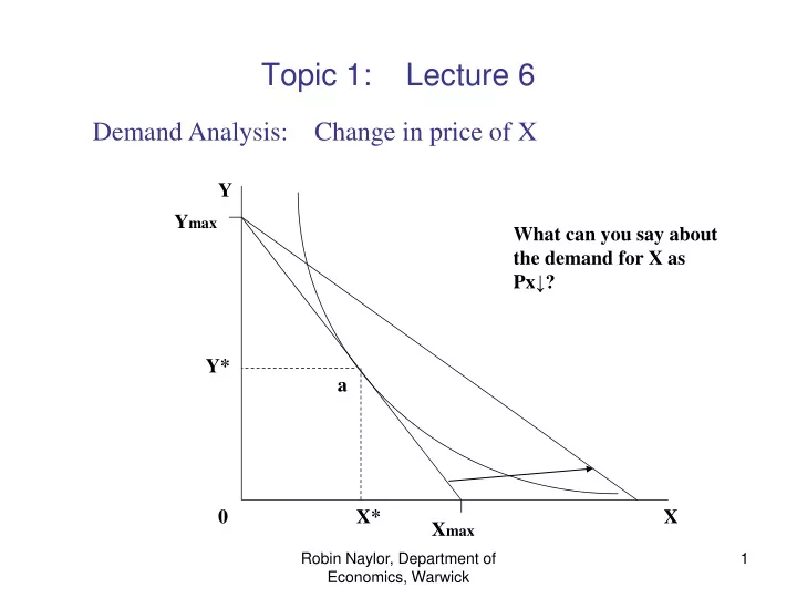
Topic 1: Lecture 6. Demand Analysis: Change in price of X. Y. Y max. What can you say about the demand for X as Px ↓?. Y*. a. 0. X*. X. X max. Topic 1: Lecture 6. Demand Analysis: Change in price of X (CASE 1). IC1. IC2. Y. Y max.

E N D
Topic 1: Lecture 6 Demand Analysis: Change in price of X Y Ymax What can you say about the demand for X as Px↓? Y* a 0 X* X Xmax Robin Naylor, Department of Economics, Warwick
Topic 1: Lecture 6 Demand Analysis: Change in price of X (CASE 1) IC1 IC2 Y Ymax What can you say about the demand for X as Px↓? â Y* a 0 X* X Xmax Robin Naylor, Department of Economics, Warwick
Topic 1: Lecture 6 Demand Analysis: Change in price of X (CASE 1) What is the implication for the shape of the demand curve for X: in (Px, X)–space? What is held constant along this demand curve? IC1 IC2 Y Ymax â Y* a 0 X* X Xmax Robin Naylor, Department of Economics, Warwick
Topic 1: Lecture 6 Demand Analysis: Change in price of X (CASE 2) What is the implication for the shape of the demand curve for X: in (Px, X)–space? What is held constant along this demand curve? IC1 Y Ymax IC2 Y* a â 0 X* X Xmax Robin Naylor, Department of Economics, Warwick
Topic 1: Lecture 6 Demand Analysis: Change in price of X (CASE 2) IC1 Y Ymax What is the relationship between the price of X, its demand, and the demand for Y? IC2 Y* a â 0 X* X Xmax Robin Naylor, Department of Economics, Warwick
Topic 1: Lecture 6 Demand Analysis: Change in price of X (CASE 3) IC1 Y IC2 Ymax What is the implication for the shape of the demand curve for X: in (Px, X)–space? â Y* a 0 X* X Xmax Robin Naylor, Department of Economics, Warwick
Topic 1: Lecture 6 Demand Analysis: Change in price of X (CASE 3) IC1 Y IC2 Ymax What is the relationship between the price of X, its demand, and the demand for Y? â Y* a 0 X* X Xmax Robin Naylor, Department of Economics, Warwick
Topic 1: Lecture 6 Demand Analysis: Change in price of X (CASE 4) IC1 IC2 Y Ymax What is the implication for the shape of the demand curve for X: in (Px, X)–space? â Y* a 0 X* X Xmax Robin Naylor, Department of Economics, Warwick
Topic 1: Lecture 6 Demand Analysis: Change in price of X (CASE 3 Revisited) • There are 2 reasons for the rise in demand for X following the fall in its price: • Disposable (or ‘real’) Income Effect • Relative Price Effect Y Ymax â Y* a 0 X* X Xmax Robin Naylor, Department of Economics, Warwick
Topic 1: Lecture 6 Demand Analysis: Change in price of X (CASE 3 Revisited) • There are 2 reasons for the rise in demand for X following the fall in its price: • Disposable (or ‘real’) Income Effect • The budget constraint shifts outwards and hence the individual can achieve higher ‘utility’; that is, move on to previously unobtainable Indifference Curves. They are able to buy more of both X and Y: whether or not they do so will depend on their preferences over X and Y. If X is normal, for example, the Real Income Effect will cause the individual to buy more X. • Relative Price Effect • X is now relatively cheaper than previously relative to Y. The individual is therefore likely to switch from Y towards X, to some extent. Robin Naylor, Department of Economics, Warwick
Topic 1: Lecture 6 Demand Analysis: Change in price of X (CASE 3 Revisited) • We would now like to be able to distinguish between these two effects in the diagram. • Real Income Effect • Relative Price Effect Y Ymax â Y* a 0 X* X Xmax Robin Naylor, Department of Economics, Warwick
Topic 1: Lecture 6 Demand Analysis: Change in price of X (CASE 3 Revisited) Consider first the Relative Price Effect. Suppose relative prices had changed, but that there had been no Real Income Effect of the price change. What point in the diagram could represent such a position? Y Ymax â Y* a 0 X* X Xmax Robin Naylor, Department of Economics, Warwick
Topic 1: Lecture 6 Demand Analysis: Change in price of X (CASE 3 Revisited) Consider first the Relative Price Effect. Suppose relative prices had changed, but that there had been no Real Income Effect of the price change. What point in the diagram could represent such a position? ‘b’ Y Ymax â Y* a b 0 X* X Xmax Robin Naylor, Department of Economics, Warwick
Topic 1: Lecture 6 Demand Analysis: Change in price of X (CASE 3 Revisited) Relative Price Effect. What change is causing the consumer equilibrium to move from ‘a’ to ‘b’? What is not changing between ‘a’ and ‘b’? Hence, ‘a’ to ‘b’ represents a pure relative price effect. Y Ymax â Y* a b As ‘a’ and ‘b’ lie on the same IC, there is no ‘Real Income’ change in moving from ‘a’ to ‘b’. 0 X* X Xmax Robin Naylor, Department of Economics, Warwick
Topic 1: Lecture 6 Demand Analysis: Change in price of X (CASE 3 Revisited) Relative Price Effect. ‘a’ to ‘b’ represents a pure relative price effect. More commonly, we refer to it as a substitution effect Y Ymax â Y* a b S 0 X* Xs X Xmax Robin Naylor, Department of Economics, Warwick
Topic 1: Lecture 6 Demand Analysis: Change in price of X (CASE 3 Revisited) Real Income Effect. We claimed that the Total Effect of the price change (i.e., from ‘a’ to ‘â’) is made up of a Relative Price (Substitution) Effect and a Real Income Effect. Y Ymax â Y* a b As ‘a’ to ‘b’ is the substitution effect, can we show that ‘b’ to ‘â’ is the Real Income Effect? S 0 X* Xs X Xmax Robin Naylor, Department of Economics, Warwick
Topic 1: Lecture 6 Demand Analysis: Change in price of X (CASE 3 Revisited) Real Income Effect. Compare ‘b’ and ‘â’. What have they got in common? What is different between them? Your answers should confirm for you that ‘b’ to ‘â’ captures the Real Income Effect. Y Ymax â Y* a b As ‘a’ to ‘b’ is the substitution effect, can we show that ‘b’ to ‘â’ is the Real Income Effect? S I 0 X* Xs X** X Robin Naylor, Department of Economics, Warwick
Topic 1: Lecture 6 Now read B&B 4th Ed., pp. 151-171 (but don’t worry about issues (especially the mathematical material) which go beyond what you have seen in lecture notes or seminar exercise sheets) Robin Naylor, Department of Economics, Warwick