Download
1 / 25
250 likes | 436 Views
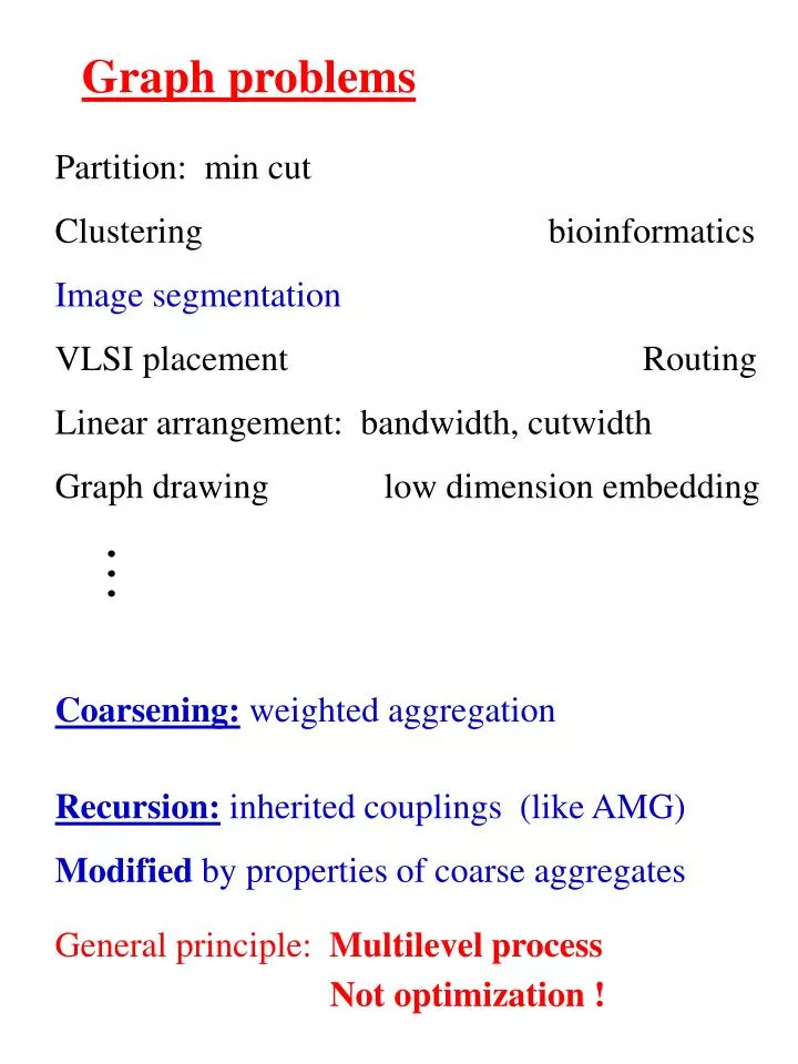
Graph problems. Partition: min cut Clustering bioinformatics Image segmentation VLSI placement Routing Linear arrangement: bandwidth, cutwidth Graph drawing low dimension embedding.

E N D
Graph problems Partition: min cut Clustering bioinformatics Image segmentation VLSI placement Routing Linear arrangement: bandwidth, cutwidth Graph drawing low dimension embedding Coarsening: weighted aggregation Recursion: inherited couplings (like AMG) Modified by properties of coarse aggregates General principle: Multilevel process Not optimization !
Multigrid solversCost: 25-100 operations per unknown Linear scalar elliptic equation (~1971)* Nonlinear Grid adaptation General boundaries, BCs* Discontinuous coefficients Disordered: coefficients, grid (FE) Several coupled PDEs* Non-elliptic: high-Reynolds flow Highly indefinite: waves Many eigenfunctions (N) Near zero modes Gauge topology: Dirac eq. Inverse problems Optimal design Integral equations Statistical mechanics Monte-Carlo Massive parallel processing *Rigorous quantitative analysis (1986)
u given on the boundary h Probability distribution of u= function ofu's andf u= function ofu's andf Point-by-point RELAXATION Point-by-point MONTE CARLO
Monte Carlocost ~ - e z 2 L Multiscale cost ~ DiscretizationLattice for accuracy “volume factor” “critical slowing down” Statistical samples Multigrid cycles Many sampling cycles at coarse levels
Scale-born obstacles: • Many variables n gridpoints / particles / pixels / … • Interacting with each otherO(n2) • Slowness Slowly converging iterations / Slow Monte Carlo / Small time steps / … 1. Localness of processing 2. Attraction basins • Multiple solutions Inverse problems / Optimization Many eigenfunctions Statistical sampling Removed by multiscale algorithms
Repetitive systemse.g., same equations everywhere UPSCALING: Derivation of coarse equationsin small windows Vs. COARSENING: For acceleration Or surrogate problems Etc.
A solution valueis NOT generally determined just by few local equations A coarse equationIS generally determined just by few local equations N unknowns O (N) solution operations UPSCALING: The coarse equation can be derived ONCE for all similar neighborhoods # operations << N
Systematic Upscaling • Choosing coarse variables • Constructing coarse-leveloperational rules equations Hamiltonian
Macromolecule ~ 10-15 second steps
ALGEBRAIC MULTIGRID (AMG) 1982 Ax = b Coarse variables - a subset Criterion: Fast convergence of “compatible relaxation” Relax Ax = 0 Keeping coarse variables = 0
Systematic Upscaling • Choosing coarse variablesCriterion: Fast convergence of “compatible relaxation” OR: Fast equilibration of “compatible Monte Carlo” Local dependence on coarse variables 2. Constructing coarse-leveloperational rules (equations / Hamiltonian) Done locally In representative “windows”
Macromolecule ~ 10-15 second steps
Macromolecule Two orders of magnitude faster simulation
t Macromolecule Dihedral potential G2 G1 T t -p 0 p + Lennard-Jones + Electrostatic ~104Monte Carlo passes for one T Gi transition
Total mass • Total momentum • Total dipole moment • average location Fluids
1 1 • 2
Windows Coarser level Larger density fluctuations Still coarser level
Total mass: Fluids Summing
Lower Temperature T Summing also Still lower T: More precise crystal direction and periods determined at coarser spatial levels Heisenberg uncertainty principle: Better orientational resolution at larger spatial scales
Optimization byMultiscale annealing Identifying increasingly larger-scale degrees of freedom at progressively lower temperatures Handling multiscale attraction basins E(r) r
Systematic Upscaling Rigorous computational methodology to derive from physical laws at microscopic (e.g., atomistic) level governing equations at increasingly larger scales. Scales are increased gradually (e.g., doubled at each level) with interscale feedbacks, yielding: • Inexpensive computation : needed only in some small “windows” at each scale. • No need to sum long-range interactions • Efficient transitions between meta-stable configurations. Applicable to fluids, solids, macromolecules, electronic structures, elementary particles, turbulence, …
Upscaling Projects • QCD (elementary particles):Renormalization multigrid RonBAMG solver of Dirac eqs. Livne, Livshits Fast update of , det Rozantsev • (3n +1) dimensional Schrödinger eq. FilinovReal-time Feynmann path integrals Zlochinmultiscale electronic-density functional • DFT electronic structures Livne, Livshits molecular dynamics • Molecular dynamics:Fluids Ilyin, Suwain, MakedonskaPolymers, proteins Bai, KlugMicromechanical structures ???defects, dislocations, grains • Navier Stokes Turbulence McWilliamsDinar, Diskin