Download
1 / 65
650 likes | 785 Views
Lecture 17 The applications of tomography: LTAO, MCAO, MOAO, GLAO. Claire Max AY 289 UC Santa Cruz March 7, 2013. Outline of lecture. What is AO tomography? AO applications of tomography Laser tomography AO Multi-conjugate AO (MCAO) Multi-object AO (MOAO) Ground-layer AO (GLAO)

E N D
Lecture 17The applications of tomography:LTAO, MCAO, MOAO, GLAO Claire Max AY 289 UC Santa Cruz March 7, 2013
Outline of lecture • What is AO tomography? • AO applications of tomography • Laser tomography AO • Multi-conjugate AO (MCAO) • Multi-object AO (MOAO) • Ground-layer AO (GLAO) • Much of this lecture is based on presentations by Don Gavel, Lisa Poyneer, and Olivier Guyon. Thanks!
Limitations for AO systems with one guide star Isoplanatic Angle Limits the corrected field r0 h θ0 3
Limitations for AO systems with one guide star Cone effect 4
Limitations for AO systems with one guide star Cone effect Missing turbulence outside and above cone Spherical wave “stretching” of wavefront More severe for larger telescope diameters r0 h 5
Fundamental problem to solve: Isoplanatic Angle If we assume perfect on-axis correction, and a single turbulent layer at altitude h, the variance (sq. radian) is : σ2 = 1.03 (θ/θ0)5/3 Where α is the angle to the optical axis, θ0 is the isoplanatic angle: θ0= 0.31 (r0/h) D = 8 m, r0 = 0.8 m, h = 5 km => θ0= 10” h
Fundamental problem to solve: Isoplanatic Angle If we assume perfect on-axis correction, and a single turbulent layer at altitude h, the variance (sq. radian) is : σ2 = 1.03 (θ/θ0)5/3 Where α is the angle to the optical axis, θ0 is the isoplanatic angle: θ0= 0.31 (r0/h) D = 8 m, r0 = 0.8 m, h = 5 km => θ0= 10” h
Francois Rigaut’s diagrams of tomography for AO 90 km “Missing” Data Credit: Rigaut, MCAO for Dummies
What is Tomography ?2. Wider field of view, no cone effect Tomography lets you reconstruct turbulence in the entire cylinder of air above the telescope mirror 90 km Credit: Rigaut, MCAO for Dummies
Concept of a metapupil • Can be made larger than “real” telescope pupil • Increased field of view due to overlap of fields toward multiple guide stars
How tomography works: from Don Gavel kZ kX Fourier slice theorem in tomography (Kak, Computer Aided Tomography, 1988) • Each wavefront sensor measures the integral of index variation along the ray lines • The line integral along z determines the kz=0 Fourier spatial frequency component • Projections at several angles sample the kx,ky,kz volume 11
How tomography works: from Don Gavel kZ kX • The larger the telescope’s primary mirror, the wider the range of angles accessible for measurement • In Fourier space, this means that the “bow-tie” becomes wider • More information about the full volume of turbulence above the telescope 12
How tomography works: some math Assume we measure y with our wavefront sensors Want to solve for x= value of δ(OPD) The equations are underdetermined – there are more unknown voxel values than measured phases ⇒ blind modes. Need a few natural guide stars to determine these. • where • y= vector of all WFS measurements • x= value of δ(OPD) at each voxel in turbulent volume above telescope x y • Ais a forward propagator
Solve for the full turbulence above the telescope using the back-propagator x • y= vector of all WFS measurements • x= value of δ(OPD) at each voxel in turbulent volume above telescope y • ATis a back propagatoralong rays back toward the guidestars x • Use iterative algorithms to converge on the solution. y
LGS Related Problems: “Null modes” • Tilt Anisoplanatism : Low order modes (e.g. focus) > Tip-Tilt at altitude • → Dynamic Plate Scale changes • Five “Null Modes” are not seen by LGS (Tilt indetermination problem) → Need 3 well spread NGSs to control these modes Credit: Rigaut, MCAO for Dummies
Outline of lecture • Review of AO tomography concepts • AO applications of tomography • Laser tomography AO • Multi-conjugate AO (MCAO) • Multi-object AO (MOAO) • Ground-layer AO (GLAO)
The multi-laser guide star AO zoo (1) Narrow field, cone effect fixed Narrow field, suffers from cone effect
The multi-laser guide star AO zoo (2) Both correct over a wide field, at a penalty in peak Strehl
The multi-laser guide star AO zoo (3) Correct over narrow field of view located anywhere w/in wide field of regard Quite modest correction over a very wide field of view
MCAO on-sky performance MCAO improves image quality where there is no single nearby bright guide star Central parts of the globular cluster Omega Centauri, as seen using different adaptive optics techniques. The upper image is a reproduction of ESO Press Photo eso0719, with the guide stars used for the MCAO correction identified with a cross. A box shows a 14 arcsec area that is then observed while applying different or no AO corrections, as shown in the bottom images. From left to right : No Adaptive Optics, Single Conjugate and Multi-Conjugate Adaptive Optics corrections. SCAO has almost no effect in sharpening the star images while the improvement provided by MCAO is remarkable. Credit: ESO
Outline of lecture • Review of AO tomography concepts • AO applications of tomography • Multi-conjugate adaptive optics (MCAO) • Multi-object adaptive optics (MOAO) • Ground-layer AO (GLAO)
What is multiconjugate AO? Turbulence Layers Deformable mirror Credit: Rigaut, MCAO for Dummies
What is multiconjugate AO? Deformable mirrors Turbulence Layers Credit: Rigaut, MCAO for Dummies
The multi-conjugate AO concept Turb. Layers Telescope WFS #2 #1 DM2 DM1 Atmosphere UP Credit: Rigaut, MCAO for Dummies
Difference between Laser Tomography AO and MCAO • Laser Tomography AO can be done with only 1 deformable mirror • If used with multiple laser guide stars, reduces cone effect • MCAO uses multiple DMs, increases field of view
“Star Oriented” MCAO Guide Stars High Altitude Layer Ground Layer Telescope DM2 DM1 WFC WFSs • Each WFS looks at one star • Global Reconstruction • n GS, n WFS, m DMs • 1 Real Time Controller • The correction applied at each DM is computed using all the input data. Credit: N. Devaney
Layer Oriented MCAO Guide Stars High Alt. Layer Ground Layer Telescope DM2 DM1 WFC1 WFC2 WFS1 WFS2 • Layer Oriented WFS architecture • Local Reconstruction • x GS, n WFS, n DMs • n RTCs • Wavefront is reconstructed at each altitude independently. • Each WFS is optically coupled to all the others. • GS light co-added for better SNR. Credit: N. Devaney
MCAO Simulations, 3 laser guide stars Strehl at 2.2μm 3 NGS, FoV = 1 arc min Strehl at 2.2μm 3 NGS, FoV = 1.5 arc min As field of view increases, average Strehl drops and variation over field increases Credit: N. Devaney
VLT Multi-conjugate AO Demonstrator (MAD) showed that MCAO works • Originally built as a technical demo to exercise in the lab, and then on the sky • Compare layer-oriented with star-oriented MCAO • Uses natural guide stars Users love it! Became a regular VLT instrument
Results from ESO’s Multiconjugate AO Demonstrator (MAD) Effective θ0 ~ 20” Effective θ0 ~ 40-50” Single Conjugate Multi Conjugate
Science papers with MAD: Orion star cluster • MCAO correction is clearly better than single conjugate AO, but this is the case all across the image (not clear what θ0 is doing)
Jupiter with MAD: single conjugate AO has done as well or better than MCAO MAD MCAO Regular Keck AO Jupiter is about 30” across
Early impressions of MCAO performance based on MAD results to date • Can extend θ0 from ~ 20 arc sec all the way to ~ 60” • Some penalty in peak Strehl, in return for larger corrected field • But really need three guide stars - hard to find if using “real” stars. (Hence MAD’s lopsided Strehl maps.) • MCAO should really excel with laser guide stars • Gemini South’s GEMS is first to do this • Note: Solar AO has demonstrated benefits of MCAO using multiple “regions of interest” as wavefront references
Orion star forming region: • Compare GEMS MCAO with ALTAIR single conjugate AO on Gemini North Telescope ALTAIR GEMS
Outline of lecture • Review of AO tomography concepts • AO applications of tomography • Multi-conjugate adaptive optics (MCAO) • Multi-object adaptive optics (MOAO) • Ground-layer AO (GLAO)
Distinctions between multi-conjugate and multi-object AO ? 1-2 arc min • DMs conjugate to different altitudes in the atmosphere • Guide star light is corrected by DMs before its wavefront is measured • Only one DM per object, conjugate to ground • Guide star light doesn’t bounce off small MEMS DMs in multi-object spectrograph
Multi-Object AO • Correct over multiple narrow fields of view located anywhere w/in wide field of regard • In most versions, each spectrograph or imager has its own MEMS AO mirror, which laser guide star lights doesn’t bounce off of • Hence this scheme is called “open loop”: DM doesn’t correct laser guide star wavefronts before LGS light goes to wavefront sensors • In one version, each LGS also has its own MEMS correction
Science with MOAO: multiple deployable spatially resolved spectrographs • A MEMS DM underneath each high-redshift galaxy, feeding a narrow-field spatially resolved spectrograph (IFU) • No need to do AO correction on the blank spaces between the galaxies
Why does MOAO work if there is only one deformable mirror in the science path? • Tomography lets you measure the turbulence throughout the volume above the telescope 90 km
Why does MOAO work if there is only one deformable mirror in the science path? • Tomography lets you measure the turbulence throughout the volume above the telescope • In the direction to each galaxy, you can then project out the turbulence you need to cancel out for that galaxy 90 km
Existing and Near-Term MOAO Systems • CANARY (Durham, Obs. de Paris, ONERA, ESO) • MOAO demonstrator for E-ELT • On William Herschel Telescope; one arm • Had already commissioning run • First NGS (done), then Rayleigh guide stars • RAVEN (U Victoria, Subaru, INO, Canadian NRC) • And Celia Blain! • MOAO demonstrator for Subaru telescope • 3 NGS wavefront sensors • Field of regard > 2.7 arc min • Will feed an IR science camera • Delivery in 2012
VILLAGES at Lick Observatory: Demonstration of Open-Loop Performance • Initial demonstration of open-loop MEMS performance • VILLAGES experiment on 1-meter telescope at Mount Hamilton (Lick Observatory) • It works!
Both E-ELT and TMT have done early designs for MOAO systems • Artist’s sketch of EAGLE MOAO system for E-ELT • One of the constraints is that the spectrographs are very large! • Hard (and expensive) to fit in a lot of them