Download

1 / 28
280 likes | 610 Views
Graph Traversals. Algorithm : Design & Analysis [14]. In the last class …. Implementing Dynamic Set by Union-Find Straight Union-Find Making Shorter Tree by Weighted Union Compressing Path by Compressing-Find Amortized Analysis of wUnion and cFind. Graph Traversals.

E N D
Graph Traversals Algorithm : Design & Analysis [14]
In the last class… • Implementing Dynamic Set by Union-Find • Straight Union-Find • Making Shorter Tree by Weighted Union • Compressing Path by Compressing-Find • Amortized Analysis of wUnion and cFind
Graph Traversals • Depth-First and Breadth-First Search • Finding Connected Components • General Depth-First Search Skeleton • Depth-First Search Trace
Graph Traversal: an Example Starting node D A Not reachable B G Breadth-First Search Starting node F C E D A Depth-First Search B G Edges only “checked” F C E Not reachable
Outline of Depth-First Search • dfs(G,v) • Mark v as “discovered”. • For each vertex w that edge vw is in G: • If w is undiscovered: • dfs(G,w) • Otherwise: • “Check” vw without visiting w. • Mark v as “finished”. That is: exploring vw, visiting w, exploring from there as much as possible, and backtrack from w to v.
Implementing Breadth-First Search Using a Queue • Input: G, a graph with n nodes, represented by an adjacency list; s, the starting vertex • Output: A breadth-first spanning tree, stored in a array • void breadthFirstSearch(intList[ ] adjVertices, intn, ints, int[ ]parent) • int[ ] color=newint[n+1]; • Queuepending=create(n); • Initialize color[1], …, color[n] to white • <the procedure, to be showed in the next frame>
Breadth-First Search: the Procedure Color tag: white: undiscovered gray: in the queue black: processed • parent[s]=-1; • color[s]=gray; • enqueue(pending, s); • while (pending is nonempty) • v=front(pending); • dequeue(pending); • for each vertex w in the list adjVertices[v]: • If (color[w]==white) • color[w]=gray; • enqueue(pending, w); • parent[w]=v; //Process tree edge vw • //Continue through list • //Process vertex v here • color[v]=black; • return
Depth-First vs. Breadth-First • Processing order • Depth-first: LIFO ( as to backtracking) • Breadth-first: FIFO (“level” by “level”) • Processing Opportunities for a node • Depth-first: 2 • At discovering • At finishing • Breadth-first: only 1, when dequeued
Depth-First Search Forward • In depth-first search, the direction of an exploration is in edge direction. • If nontree edges will be ignored, the undirected graph to be depth-first searched can be substituted by symmetric digraph. • Backward search can be implemented as easily as forward, using transpose graph GT, which simply results from reversing the direction of each edge in G.
Depth-First Search and Recursion This is the last to do result processing 1 6 The order of the execution of recursive calls, which is different from the order of result processing 2 17 5 4 3 23 18 12 4 3 3 2 16 13 22 19 4 9 1 3 2 2 2 1 1 0 24 25 8 20 5 15 21 2 1 1 0 1 0 1 0 14 11 10 6 7 1 0 Fibonacci: Fn= Fn-1+Fn-2,by recursion
Backtrack Searching Start (1,1) (1,2) (1,3) (1,4) (1,5) (1,6) (1,7) (1,8) (2,3) (2,4)(2,5)(2,6)(2,7)(2,8) The Eight Queen Problem (3,5)(3,6)(3,7)(3,8) Nodes are labeled by the location codes on the chess borad in which a queen may be place. (4,2) (4,7) (4,8) (5,4)(5,8) Dead end: backtrack occurs
Finding Connected Components • Input: a symmetric digraph G, with n nodes and 2m edges(interpreted as an undirected graph), implemented as a array adjVerteces[1,…n] of adjacency lists. • Output: an array cc[1..n] of component number for each node vi • void connectedComponents(Intlist[ ] adjVertices, intn, int[ ] cc)//This is a wraaper procedure • int[ ] color=newint[n+1]; • int v; • <Initialize color array to white for all vertices> • for (v=1; vn; v++) • if (color[v]==white) • ccDFS(adjVertices, color, v, v, cc); • return Depth-first search
ccDFS: the procedure • void ccDFS(IntList[ ] adjVertices, int[ ] color, intv, intccNum, int [ ] cc)//v as the code of current connected component • int w; • IntList remAdj; • color[v]=gray; • cc[v]=ccNum; • remAdj=adjVertices[v]; • while (remAdjnil) • w=first(remAdj); • if(color==white) • ccDFS(adjVertices, color, w, ccNum, cc); • remAdj=rest(remAdj); • color[v]=black; • return The elements of remAdj are neighbors of v Processing the next neighbor, if existing, another depth-first search to be incurred v finished
Analysis of Connected Components Algorithm • connectedComponents, the wrapper • Linear in n (color array initialization+for loop on adjVertices ) • ccDFS, the depth-first searcher • In one execution of ccDFS on v, the number of instructions(rest(remAdj)) executed is proportional to the size of adjVertices[v]. • Note: (size of adjVertices[v]) is 2m, and theadjacency lists are traveresed only once. • So, the complexity is in (m+n) • Extra space requirements: • color array • activation frame stack for recursion
Depth-First Search Trees DFS forest={(DFS tree1), (DFS tree2)} Root of tree 1 B.E D A T.E C.E T.E B.E B G D.E C.E C.E T.E T.E T.E: tree edge B.E: back edge D.E: descendant edge C.E: cross edge T.E F C E C.E C.E Root of tree 2 A finished vertex is never revisited, such as C
Visits On a Vertex • Classification for the visits on a vertex • First visit(exploring): status: whitegray • (Possibly) multi-visits by backtracking to: status keeps gray • Last visit(no more branch-finished): status: grayblack • Different operations can be done on the vertex or (selected) incident edges during the different visits on a specific vertex
Depth-First Search: Generalized • Input: Array adjVertices for graph G • Output: Return value depends on application. • int dfsSweep(IntList[] adjVertices,int n, …) • intans; • <Allocate color array and initialize to white> • For each vertex v of G, in some order • if (color[v]==white) • int vAns=dfs(adjVertices, color, v, …); • <Process vAns> • // Continue loop • return ans;
Depth-First Search: Generalized If partial search is used for a application, tests for termination may be inserted here. • int dfs(IntList[] adjVertices, int[] color, int v, …) • int w; • IntList remAdj; • int ans; • color[v]=gray; • <Preorder processing of vertex v> • remAdj=adjVertices[v]; • while (remAdjnil) • w=first(remAdj); • if (color[w]==white) • <Exploratory processing for tree edge vw> • int wAns=dfs(adjVertices, color, w, …); • < Backtrack processing for tree edge vw , using wAns> • else • <Checking for nontree edge vw> • remAdj=rest(remAdj); • <Postorder processing of vertex v, including final computation of ans> • color[v]=black; • return ans; • Specialized for connected components: • parameter added • preorder processing inserted – cc[v]=ccNum
Time Relation on Changing Color • Keeping the order in which vertices are encountered for the first or last time • A global integer time: 0 as the initial value, incremented with each color changing for any vertex, and the final value is 2n • Array discoverTime: the i th element records the time vertex vi turns into gray • Array finishTime: the i th element records the time vertex vi turns into black • The active interval for vertex v, denoted as active(v), is the duration while v is gray, that is: discoverTime[v], …, finishTime[v]
Depth-First Search Trace • General DFS skeleton modified to compute discovery and finishing times and “construct” the depth-first search forest. • int dfsTraceSweep(IntList[ ] adjVertices,int n, int[ ] discoverTime, int[ ] finishTime, int[ ] parent) • intans; int time=0 • <Allocate color array and initialize to white> • For each vertex v of G, in some order • if (color[v]==white) • parent[v]=-1 • int vAns=dfsTrace(adnVertices, color, v, discoverTime, finishTime, parent, time); • // Continue loop • return ans;
Depth-First Search Trace • int dfsTrace(IntList[ ] adjVertices, int[ ] color, int v, int[ ] discoverTime,int[ ] finishTime, int[ ] parent int time) • int w; • IntList remAdj; • int ans; • color[v]=gray; • time++; discoverTime[v]=time; • remAdj=adjVertices[v]; • while (remAdjnil) • w=first(remAdj); • if (color[w]==white) • parent[w]=v; • int wAns=dfsTrace(adjVertices, color, w, discoverTime, finishTime, parent, time); • else • <Checking for nontree edge vw> • remAdj=rest(remAdj); • time++; finishTime[v]=time; • color[v]=black; • return ans;
Edge Classification and the Active Intervals 1/10 5/6 B.E D A T.E C.E T.E 2/7 B.E 12/13 B G D.E C.E The relations are summarized in the next frame C.E T.E T.E T.E F C E 8/9 C.E C.E 11/14 3/4 Time 1 2 3 4 5 6 7 8 9 10 11 12 13 14 A E G B F C D
Properties about Active Intervals(1) • If w is a descendant of v in the DFS forest, then active(w)active(v), and the inclusion is proper if wv. • Proof: • Define a partial order <: w<v iff. w is a proper descentants of v in its DFS tree. The proof is by induction on <) • If v is minimal. The only descendant of v is itself. Trivial. • Assume that for all x<v, if w is a descendant of x, then active(w)active(x). • Let w is any proper descendant of v in the DFS tree, there must be some x such that vx is a tree edge on the tree path to w, so w is a descendant of x. According to dfsTrace, we have active(x)active(v), by inductive hypothesis, active(w)active(v),
Properties about Active Intervals(2) • If v and w have no ancestor/descendant relationship in the DFS forest, then their active intervals are disjoint. • Proof: • If v and w are in different DFS tree, it is triavially true, since the trees are processed one by one. • Otherwise, there must be a vertex c, satisfying that there are tree paths c to v, and c to w, without edges in common. Let the leading edges of the two tree path are cy, cz, respectively. According to dfsTrace, active(y) and active(z) are disjoint. • We have active(v)active(y), active(w)active(z). So, active(v) and active(w) are disjoint.
Properties about Active Intervals(3) • If active(w)active(v), then w is a descendant of v. And if active(w)active(v), then w is a proper descendant of v. • Proof: • If w is not a descendant of v, there are two cases: • v is a proper descendant of w, then active(v)active(w), so, it is impossible that active(w)active(v), contradiction. • There is no ancestor/descendant relationship between v and w, then active(w) and active(v) are disjoint, contradiction.
Properties about Active Intervals(4) • If edge vwEG, then • vw is a cross edge iff. active(w) entirely precedes active(v). • vw is a descendant edge iff. there is some third vertex x, such that active(w)active(x)active(v), • vw is a tree edge iff. active(w)active(v), and there is no third vertex x, such that active(w)active(x) active(v), • vw is a back edge iff. active(v)active(w),
DFS Tree Path • [White Path Theorem] w is a descendant of v in a DFS tree iff. at the time v is discovered (just to be changing color into gray), there is a path in G from v to w consisting entirely of white vertices. • Proof • All the vertices in the path are descendants of v. • by induction on the length k of a white path from v to w. • When k=0, v=w. • For k>0, let P(v, x1,x2,…xk=w). There must be some vertex on P which is discovered during the active interval of v, e.g. x1, Let xi is earliest discovered among them. Divide P into P1 from v to xi, and P2 from xi to w. P2 is a white path with length less than k, so, by inductive hypothesis, w is a descendant of xi. Note: active(xi)active(v), so xi is a descendant of v. By transitivity, w is a descendant of v.
Home Assignments • 7.12 • 7.14 • 7.15 • 7.16