Topology Control in Ad hoc and Sensor Networks

1. Ad hoc and Sensor NetworksChapter 10: Topology control Holger Karl

2. Goals of this chapter • Networks can be too dense – too many nodes in close (radio) vicinity • This chapter looks at methods to deal with such networks by • Reducing/controlling transmission power • Deciding which links to use • Turning some nodes off • Focus is on basic ideas, some algorithms • Complexity results are only very superficially covered Ad hoc & sensor networs - Ch 10: Topology control

3. Overview • Motivation, basics • Power control • Backbone construction • Clustering • Adaptive node activity Ad hoc & sensor networs - Ch 10: Topology control

4. Motivation: Dense networks • In a very dense networks, too many nodes might be in range for an efficient operation • Too many collisions/too complex operation for a MAC protocol, too many paths to chose from for a routing protocol, … • Idea: Make topology less complex • Topology: Which node is able/allowed to communicate with which other nodes • Topology control needs to maintain invariants, e.g., connectivity Ad hoc & sensor networs - Ch 10: Topology control

5. Topology Control Drop long-range neighbors: Reduces interference and energy! But still stay connected (or even spanner) Ad hoc & sensor networs - Ch 10: Topology control

6. Topology Control as a Trade-Off Sometimes also clustering, dominating set construction (see later) Topology Control Network ConnectivitySpanner Property Conserve EnergyReduce Interference Sparse Graph, Low Degree Planarity Symmetric Links Less Dynamics d(u,v) ¢ t ¸ dTC(u,v) Ad hoc & sensor networs - Ch 10: Topology control

7. Options for topology control Topology control Control link activity – deliberately use/not use certain links Control node activity – deliberately turn on/off nodes Topology control Hierarchical network – assign different roles to nodes; exploit that to control node/link activity Flat network – all nodes have essentially same role Power control Backbones Clustering Ad hoc & sensor networs - Ch 10: Topology control

8. Flat networks • Main option: Control transmission power • Do not always use maximum power • Selectively for some links or for a node as a whole • Topology looks “thinner” • Less interference, … • Alternative: Selectively discard some links • Usually done by introducing hierarchies Ad hoc & sensor networs - Ch 10: Topology control

9. Hierarchical networks – backbone • Construct a backbone network • Some nodes “control” their neighbors – they form a (minimal) dominating set • Each node should have a controlling neighbor • Controlling nodes have to be connected (backbone) • Only links within backbone and from backbone to controlled neighbors are used • Formally: Given graph G=(V,E), construct D ½ V such that Ad hoc & sensor networs - Ch 10: Topology control

10. Hierarchical network – clustering • Construct clusters • Partition nodes into groups (“clusters”) • Each node in exactly one group • Except for nodes “bridging” between two or more groups • Groups can have clusterheads • Typically: all nodes in a cluster are direct neighbors of their clusterhead • Clusterheads are also a dominating set, but should be separated from each other – they form an independent set • Formally: Given graph G=(V,E), construct C ½ V such that Ad hoc & sensor networs - Ch 10: Topology control

11. Aspects of topology-control algorithms • Connectivity – If two nodes connected in G, they have to be connected in G0 resulting from topology control • Stretch factor – should be small • Hop stretch factor: how much longer are paths in G0 than in G? • Energy stretch factor: how much more energy does the most energy-efficient path need? • Throughput – removing nodes/links can reduce throughput, by how much? • Robustness to mobility • Algorithm overhead Ad hoc & sensor networs - Ch 10: Topology control

12. Example: Price for maintaining connectivity • Maintaining connectivity can be very “costly” for a power control approach • Compare power required for connectivity compared to power required to reach a very big maximum component Ad hoc & sensor networs - Ch 10: Topology control

13. Overview • Motivation, basics • Power control • Backbone construction • Clustering • Adaptive node activity Ad hoc & sensor networs - Ch 10: Topology control

14. Power control – magic numbers? • Question: What is a good power level for a node to ensure “nice” properties of the resulting graph? • Idea: Controlling transmission power corresponds to controlling the number of neighbors for a given node • Is there an “optimal” number of neighbors a node should have? • Is there a “magic number” that is good irrespective of the actual graph/network under consideration? • Historically, k=6 or k=8 had been suggested as such “magic numbers” • However, they optimize progress per hop – they do not guarantee connectivity of the graph!! ! Needs deeper analysis Ad hoc & sensor networs - Ch 10: Topology control

15. Controlling transmission range • Assume all nodes have identical transmission range r=r(|V|), network covers area A, V nodes, uniformly distr. • Fact: Probability of connectivity goes to zero if: • Fact: Probability of connectivity goes to 1 for if and only if |V|->inf. with |V| • Fact (uniform node distribution, density ): Ad hoc & sensor networs - Ch 10: Topology control

16. Controlling number of neighbors • Knowledge about range also tells about number of neighbors • Assuming node distribution (and density) is known, e.g., uniform • Alternative: directly analyze number of neighbors • Assumption: Nodes randomly, uniformly placed, only transmission range is controlled, identical for all nodes, only symmetric links are considered • Result: For connected network, required number of neighbors per node is  (log |V|) • It is not a constant, but depends on the number of nodes! • For a larger network, nodes need to have more neighbors & larger transmission range! – Rather inconvenient • Constants can be bounded Ad hoc & sensor networs - Ch 10: Topology control

17. Basic idea for most of the following methods: Take a graph G=(V,E), produce a graph G0=(V,E0) that maintains connectivity with fewer edges Assume, e.g., knowledge about node positions Construction should be local (for distributed implementation) Some example constructions for power control Ad hoc & sensor networs - Ch 10: Topology control

18. Example 1: Relative Neighborhood Graph (RNG) • Edge between nodes u and v if and only if there is no other node w that is closer to either u or v • Formally: • RNG maintains connectivity of the original graph • Easy to compute locally • But: Worst-case spanning ratio is  (|V|) • Average degree is 2.6 This region has to be empty for the two nodes to be connected Ad hoc & sensor networs - Ch 10: Topology control

19. Gabriel graph (GG) similar to RNG Difference: Smallest circle with nodes u and v on its circumference must only contain node u and v for u and v to be connected Formally: Properties: Maintains connectivity, Worst-case spanning ratio (|V|1/2), energy stretch O(1) (depending on consumption model!), worst-case degree  (|V|) Example 2: Gabriel graph This region has to be empty for the two nodes to be connected Ad hoc & sensor networs - Ch 10: Topology control

20. Edges of Delaunay triangulation Example 3: Delaunay triangulation • Assign, to each node, all points in the plane for which it is the closest node !Voronoi diagram • Constructed in O(|V| log |V|) time • Connect any two nodes for which the Voronoi regions touch !Delaunay triangulation • Problem: Might produce very long links; not well suited for power control Voronoi region for upper left node Ad hoc & sensor networs - Ch 10: Topology control

21. Spanning Tree Based Construction • Build local spanning trees • Each node collects info about its neighbors at max. Power • Construct an MST using asy Prim’s Algorithm • Use only tree topology for communication Ad hoc & sensor networs - Ch 10: Topology control

22. Finding a Spanning Tree Given a Root • a distinguished processor is known, to serve as the root • root sends M to all its neighbors • when non-root first gets M • set the sender as its parent • send "parent" msg to sender • send M to all other neighbors • when get M otherwise • send "reject" msg to sender • use "parent" and "reject" msgs to set children variables and know when to terminate Ad hoc & sensor networs - Ch 10: Topology control

23. c b b c a a f d f d e e g h g h Execution of Spanning Tree Alg. Both models: O(m) messages O(diam) time Asynchronous: not necessarily BFS tree Synchronous: always gives breadth-first search (BFS) tree Ad hoc & sensor networs - Ch 10: Topology control

24. Chang-Robert’s algorithm {The root is known} Uses signals and acks, similar to the termination detection algorithm. Uses the same rule for sending acknowledgment. Distributed Spanning tree construction For a graph G=(V,E), a spanning tree is a maximally connected subgraph T=(V,E’), E’ E,such that if one more edge is added, then the subgraph is no more a tree. Used for broadcasting in a network. Question:What if the root is not designated? Ad hoc & sensor networs - Ch 10: Topology control

25. program probe-echo define N : integer (no. of neighbors) C, D : integer; initially parent :=i; C=0; D=0; {for the initiator} send probes to each neighbor; D:=no. of neighbors; do D!=0  echo -> D:=D-1 od {D=0 signals end} { for a non-initator process i>0} do probe parent=iC=0 -> C:=1; parent := sender; ifi is not a leaf -> send probes to non – parent neighbors; D:= no. of non-parent neighbors fi;  echo -> D:=D-1;  probe  sender != parent -> send echo to sender;  C=1  D=0 -> send echo to parent; C:=0; od Chang Roberts Spanning Tree Alg Ad hoc & sensor networs - Ch 10: Topology control

26. Example: Cone-based topology control • Assumption: Distance and angle information between nodes is available • Two-phase algorithm • Phase 1 • Every node starts with a small transmission power • Increase it until a node has sufficiently many neighbors • What is “sufficient”? – When there is at least one neighbor in each cone of angle  •  = 5/6 is necessary and sufficient condition for connectivity! • Phase 2 • Remove redundant edges: Drop a neighbor w of u if there is a node v of w and u such that sending from u to w directly is less efficient than sending from u via v to w • Essentially, a local Gabriel graph construction Ad hoc & sensor networs - Ch 10: Topology control

27. /2 /2 /2 /2 /2 /2 /2 /2 Example: Cone-based topology control (2) • Properties: simple, local construction • Extensions for k-connectivity (Yao graph) • Little exercise: What happens when  < or > 5/6 ? Ad hoc & sensor networs - Ch 10: Topology control

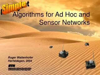
28. Centralized power control algorithm • Goal: Find topology control algorithm minimizing the maximum power used by any node • Ensuring simple or bi-connectivity • Assumptions: Locations of all nodes and path loss between all node pairs are known; each node uses an individually set power level to communicate with all its neighbors • Idea: Use a centralized, greedy algorithm • Initially, all nodes have transmission power 0 • Connect those two components with the shortest distance between them (raise transmission power accordingly) • Second phase: Remove links (=reduce transmission power) not needed for connectivity • Exercise: Relation to Kruskal’s MST algorithm? Ad hoc & sensor networs - Ch 10: Topology control

29. E E E F F F 2) Connect A-B 1) Connect A-C and B-D 4 4 3 C C C D D D 1 1 1 1 1 1 B B B A A A 2 2 E E F F 3) Connect C-D 5) Remove edge A-B 4) Connect C-E and D-F 4 4 E F 3 3 C C D D 4 4 1 1 1 1 3 C B B A A 2 1 1 B A 2 Centralized power control algorithm Topology D Ad hoc & sensor networs - Ch 10: Topology control

30. Gabriel Graph v disk(u,v) u Let disk(u,v) be a disk with diameter (u,v)that is determined by the two points u,v. The Gabriel Graph GG(V) is defined as an undirected graph (with E being a set of undirected edges). There is an edge between two nodes u,v iff the disk(u,v) including boundary contains no other points. As we will see the Gabriel Graph has interesting properties. Ad hoc & sensor networs - Ch 10: Topology control

31. Delaunay Triangulation v disk(u,v,w) w u Let disk(u,v,w) be a disk defined bythe three points u,v,w. The Delaunay Triangulation (Graph) DT(V) is defined as an undirected graph (with E being a set of undirected edges). There is a triangle of edges between three nodes u,v,w iff the disk(u,v,w) contains no other points. The Delaunay Triangulation is thedual of the Voronoi diagram, andwidely used in various CS areas;the DT is planar; the distance of apath (s,…,t) on the DT is within a constant factor of the s-t distance. Ad hoc & sensor networs - Ch 10: Topology control

32. Other planar graphs u v Relative Neighborhood Graph RNG(V) An edge e = (u,v) is in the RNG(V) iff there is no node w with (u,w) < (u,v) and (v,w) < (u,v). Minimum Spanning Tree MST(V) A subset of E of G of minimum weightwhich forms a tree on V. Ad hoc & sensor networs - Ch 10: Topology control

33. Properties of planar graphs Theorem 1: Corollary:Since the MST(V) is connected and the DT(V) is planar, all the planar graphs in Theorem 1 are connected and planar. Theorem 2:The Gabriel Graph contains the Minimum Energy Path(for any path loss exponent ¸ 2) Corollary:GG(V) Å UDG(V) contains the Minimum Energy Path in UDG(V) Ad hoc & sensor networs - Ch 10: Topology control

34. Overview • Motivation, basics • Power control • Backbone construction • Clustering • Adaptive node activity Ad hoc & sensor networs - Ch 10: Topology control

35. Hierarchical networks – backbones • Idea: Select some nodes from the network/graph to form a backbone • A connected, minimal, dominating set (MDS or MCDS) • Dominating nodes control their neighbors • Protocols like routing are confronted with a simple topology – from a simple node, route to the backbone, routing in backbone is simple (few nodes) • Problem: MDS is an NP-hard problem • Hard to approximate, and even approximations need quite a few messages Ad hoc & sensor networs - Ch 10: Topology control

36. Backbone by growing a tree • Construct the backbone as a tree, grown iteratively Ad hoc & sensor networs - Ch 10: Topology control

37. Backbone by growing a tree – Example 1: 2: 3: 4: Ad hoc & sensor networs - Ch 10: Topology control

38. Problem: Which gray node to pick? • When blindly picking any gray node to turn black, resulting tree can be very bad Solution: Look ahead! One step suffices Ad hoc & sensor networs - Ch 10: Topology control

39. Performance of tree growing with look ahead • Dominating set obtained by growing a tree with the look ahead heuristic is at most a factor 2(1+ H()) larger than MDS • H(¢) harmonic function, H(k) = i=1k 1/i <= ln k + 1 •  is maximum degree of the graph • It is automatically connected • Can be implemented in a distributed fashion as well Ad hoc & sensor networs - Ch 10: Topology control

40. Start big, make lean • Idea: start with some, possibly large, connected dominating set, reduce it by removing unnecessary nodes • Initial construction for dominating set • All nodes are initially white • Mark any node black that has two neighbors that are not neighbors of each other (they might need to be dominated) ! Black nodes form a connected dominating set (proof by contradiction); shortest path between ANY two nodes only contains black nodes • Needed: Pruning heuristics Ad hoc & sensor networs - Ch 10: Topology control

41. Pruning heuristics • Heuristic 1: Unmark node v if • Node v and its neighborhood are included in the neighborhood of some node marked node u (then u will do the domination for v as well) • Node v has a smaller unique identifier than u (to break ties) • Heuristic 2: Unmark node v if • Node v’s neighborhood is included in the neighborhood of two marked neighbors u and w • Node v has the smallest identifier of the tree nodes • Nice and easy, butonly linear approximationfactor w u v a b c d Ad hoc & sensor networs - Ch 10: Topology control

42. One more distributed backbone heuristic: Span • Construct backbone, but take into account need to carry traffic – preserve capacity • Means: If two paths could operate without interference in the original graph, they should be present in the reduced graph as well • Idea: If the stretch factor (induced by the backbone) becomes too large, more nodes are needed in the backbone • Rule: Each node observes traffic around itself • If node detects two neighbors that need three hops to communicate with each other, node joins the backbone, shortening the path • Contention among potential new backbone nodes handled using random backoff A C B Ad hoc & sensor networs - Ch 10: Topology control

43. Overview • Motivation, basics • Power control • Backbone construction • Clustering • Adaptive node activity Ad hoc & sensor networs - Ch 10: Topology control

44. Clustering • Partition nodes into groups of nodes – clusters • Many options for details • Are there clusterheads? – One controller/representative node per cluster • May clusterheads be neighbors? If no: clusterheads form an independent set C:Typically: clusterheads form a maximum independent set • May clusters overlap? Do they have nodes in common? Ad hoc & sensor networs - Ch 10: Topology control

45. Clustering • Further options • How do clusters communicate? Some nodes need to act as gateways between clustersIf clusters may not overlap, two nodes need to jointly act as a distributed gateway • How many gateways exist between clusters? Are all active, or some standby? • What is the maximal diameter of a cluster? If more than 2, then clusterheads are not necessarily a maximum independent set • Is there a hierarchy of clusters? Ad hoc & sensor networs - Ch 10: Topology control

46. Maximum independent set • Computing a maximum independent set is NP-complete • Can be approximate within ( +3)/5 for small , within O( log log  / log ) else;  bounded degree • Show: A maximum independent set is also a dominating set • Maximum independent set not necessarily intuitively desired solution • Example: Radial graph, with only (v0,vi) 2 E Ad hoc & sensor networs - Ch 10: Topology control

47. 1 1 1 1 1 2 2 2 2 2 3 3 3 3 3 7 7 7 7 7 6 6 6 6 6 5 5 5 5 5 4 4 4 4 4 Step 4: Step 2: Step 1: Init: Step 3: A basic construction idea for independent sets • Use some attribute of nodes to break local symmetries • Node identifiers, energy reserve, mobility, weighted combinations… - matters not for the idea as such (all types of variations have been looked at) • Make each node a clusterhead that locally has the largest attribute value • Once a node is dominated by a clusterhead, it abstains from local competition, giving other nodes a chance Ad hoc & sensor networs - Ch 10: Topology control

48. Determining gateways to connect clusters • Suppose: Clusterheads have been found • How to connect the clusters, how to select gateways? • It suffices for each clusterhead to connect to all other clusterheads that are at most three hops • Resulting backbone (!) is connected • Formally: Steiner tree problem • Given: Graph G=(V,E), a subset C ½ V • Required: Find another subset T ½ V such that S [ T is connected and S [ T is a cheapest such set • Cost metric: number of nodes in T, link cost • Here: special case since C are an independent set Ad hoc & sensor networs - Ch 10: Topology control

49. Steiner Tree (from Yao Wen Chang) Ad hoc & sensor networs - Ch 10: Topology control

50. Rotating clusterheads • Serving as a clusterhead can put additional burdens on a node • For MAC coordination, routing, … • Let this duty rotate among various members • Periodically reelect – useful when energy reserves are used as discriminating attribute • LEACH – determine an optimal percentage P of nodes to become clusterheads in a network • Use 1/P rounds to form a period • In each round, nP nodes are elected as clusterheads • At beginning of round r, node that has not served as clusterhead in this period becomes clusterhead with probability P/(1-p(r mod 1/P)) Ad hoc & sensor networs - Ch 10: Topology control